
The math exams of my life
Table of contents
- The system is flawed
- The system is simple
- My first important exam - Capacitate (2001)
- The second important exam - Bacalaureat (2005)
- The third exam - Admiterea la Politehnica (2005)
- Conclusions
The system is flawed
The Romanian public education system, which, by the way, is free for everyone (Universities included), has its flaws. However, it is still one of the best in the world for making a handful of kids proficient in mathematics and sciences. It’s a system of contrasts. On the one hand, you have a bunch of Elite Schools and Universities that put a lot of emphasis on scientific education, and on the other hand, you have the “average” Public Schools creating kids that can barely read, do simple arithmetics, or understand a simple text. Every middle-class parent that cares about the education of its children wants to send their children to an Elite Public School. The average school is actually below average, and Private Schools don’t have the best reputation, are too expensive, or are not that popular. The term Elite is not formalised, but there are “unofficial” rankings about how good the school is.
Getting there is mainly a meritocratic process. The child (or adolescent) must pass a few exams, and if he/she is 10/10 (or 9.50/10) he/she will be accepted almost anywhere. If you are 8.5/10, you will still get to a decent school. Lower than that, not so good. This state of affairs is similar to all the countries from the Eastern Bloc, not only Romania. So, if you speak with a Bulgarian, Hungarian, Polish, Ukrainian, or Russian person, they will tell you the same story.
This is the secret recipe for why Eastern and Central Europe is so well-represented at the International Math Olympiad. Those Elite Schools, spread in every region of the country, try to create the next generation of olimpici (kids that go to the Olympiads). Those Elite Schools are almost always Math oriented. It’s practically a cult (without any negative connotation).
Let’s look at the following table of results for IMO:
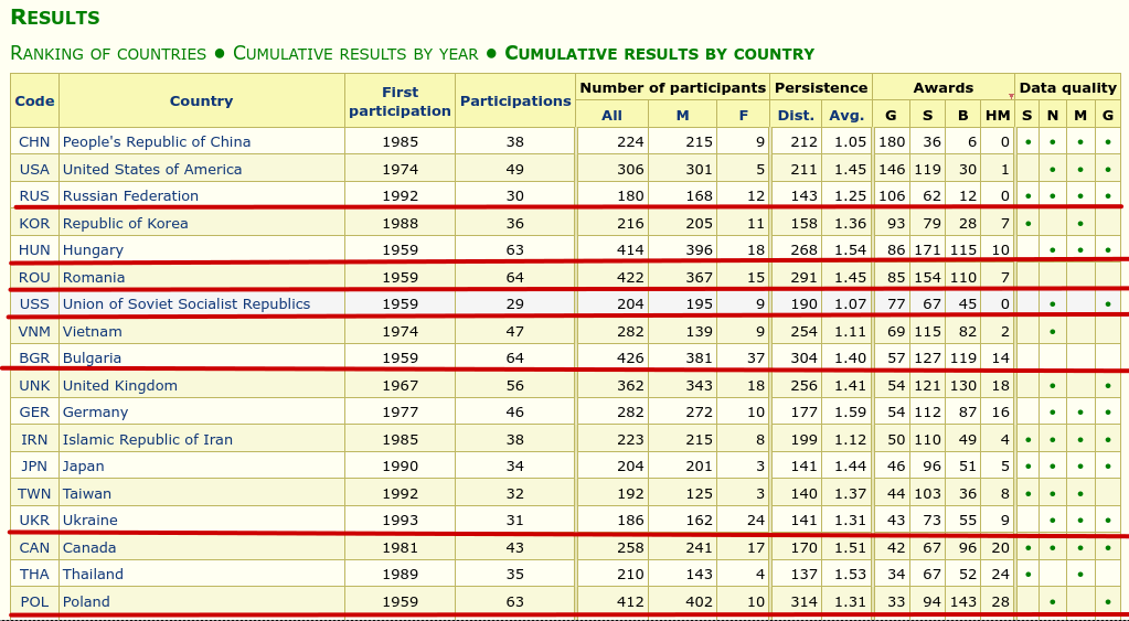
If you take Russia and Ukraine aside, Romania, Bulgaria, Hungary, and Poland have less than 80 million citizens together, but have accounted for 261 Gold Medals through the years, more than China or USA, the World’s two Superpowers. Of course, most of those students (and the ones that don’t qualify to the International but are way above the world’s average) leave Romania (or Poland, Hungary, and Bulgaria) to more prosperous, more developed countries. So what’s with all the fuss? Brain drain is a sad reality few try to counter.
The way those schools create the next-gen olimpic is simple: you make the kids take 4-6 of Math a week (or more), you give extensive Math homework (tens or hundreds of exercises per week), you ask the student to come to special classes designed to prepare them for the Olympiad, and then you repeat the formula for 12 years. Not everyone can make it, and the competition is tight. There’s a flaw here: some kids are differently wired than others and like challenges, but the constant grind is not suitable for everyone. Our Educational system is flawed because it expects almost everyone to ace Math. For example, I had colleagues in my class who are now lawyers, doctors, or work in creative industries but finished the Elite (Math) School only because the education there was so much better. So yes, in Romania, there are lawyers who studied Riemann Sums, and dentists who did prove Euler’s identity with Taylor Series. We did learn both concepts in high school, but those are not necessarily part of the standard curricula.
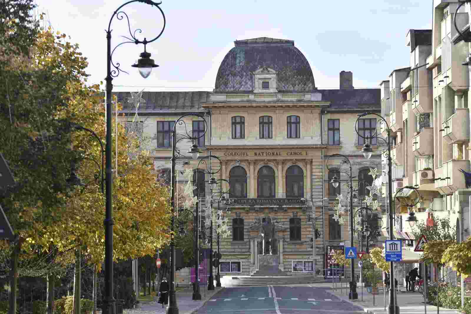
In the Romanian region where I was born (Oltenia), the elite high schools were: Colegiul National Carol I, Colegiul National Fratii Buzesti, and Colegiul National Elena-Cuza (but historically speaking, this one was focused on Humanities). I’ve picked CNC1, but the alternative would’ve been as good. I remember that one of the role models we had in our first year of high school was Mihai Patrascu (he was 3-4 years older than us), but all the teachers told us how great he is/was as a student. He was great at Computer Science and had fantastic results in Math.
In Bucharest, you can probably find even better schools, as the competition between students is more fierce. Everyone knows about Colegiul National Gheorghe Lazar, Colegiul National Sfantul Sava, or Colegiul National Tudor Vianu, a school that only in the last decade had 30 gold medalists, 53 silver medalists and 36 bronze medalists in various international competitions (mainly Math, Physics and Informatics).
The (sub)cult(ure) of Mathematics in Eastern Europe is older than communism, and the results were always notable. Communists loved Mathematics a lot. It was one of the few occupations that could instantly reward you with a decent life. It didn’t require you to scream total allegiance to the Communist Party, and it allowed you to have a few excentricities well tolerated by a dictatorial regime. So people went for it. To put it like this, Nicolae Ceasusescu’s daughter, Zoia Ceausescu, was an accomplished mathematician; even if her parents disagreed with her passion, eventually, they accepted this endeavor to be worthy of a Communist Princess. The regime did not inflate her skills in mathematics; for example, a well-regarded academician Solomon Marcus, vouched for her talent in an interview long after communism fell and Zoia died. He had no incentive to lie about the subject; it was a free country.
As a fun fact, the current mayor of Bucharest, Nicusor Dan is a two-time Gold Medalist at the International Mathematics Olympiad. He had a perfect score each time.
The system is simple
The Romanian education system is simple and shows little flexibility. It doesn’t care about too much about the children’s talents
You cannot take “extra classes”, and the first eight years of school are standard for everyone regardless of their skills and aptitudes:
- The first cycle is called Scoala Primara (Primary school). Scoala Primara is about four years (or five) years long. You start school when you are 6, 7, or 8. I started school at 6 (in 1993), but most people send their kids to school at around 7.
- The second cycle, Scoala Generala, takes four years and starts when you are around 11-12. In recent times, if you want to attend an Elite School, you must pass an admission exam. The exam is not standard, and the Elite Schools decide the curricula. Sometimes, the curricula contain topics not part of the formal curricula, so the aspiring kid has to take private tutoring to prepare for this exam.
- At the end of the Scoala Generala, you must pass another exam called Capacitate (in my time) or Teste Nationale (in recent times). This exam is the first important one. If you are close to 10/10, you will be admitted to the Elite School; anything under 9/10 makes it more difficult or impossible. The admission process is totally transparent. You cannot bribe your way into admission, or at least not in this phase of the process.
- The third cycle is Liceul. This is where diversification first appears. You can go to a Profil Real to study matematica-informatica or a Profil Uman, to study Humanities. If you pick Profil Uman, it means your mathematical education stops. Usually, the best pick is matematica-informatica, which can also be spiced up with additional hours of math, physics, or informatics (basically Computer Science).
- At the end of high school, there’s a second exam called Baccaluareat (like in France). Getting a big mark at Baccalaureat helps you get admitted to local Universities, but there’s also an admission exam for the really good ones.
My first important exam - Capacitate (2001)
It was 2001, and the first important Math exam I had to take was called Capacitate. I was 13 or 14 years old. Thanks to the internet, I did find the subjects online, so I had to solve them almost 23 years apart.
The exam was tailored to make it easy to get a mark higher than 7/10 and significantly more challenging to get a mark higher than 9/10.
Anything better than 9/10 would help you land a place in an Elite school. This was the target, so I aimed to get a perfect score (I was close: 9.80/10, if I remember correctly). Since I was ten years old, I have also participated in Math Olympiads, always making it into the top 25 students of my region (my best was 4th rank), so I remember Capacitate to be manageable.
In Scoala Generala I remember a lot of emphasis was put on basic Algebra and Geometry (2d and 3d). The student had to develop the graphical intuition of things.
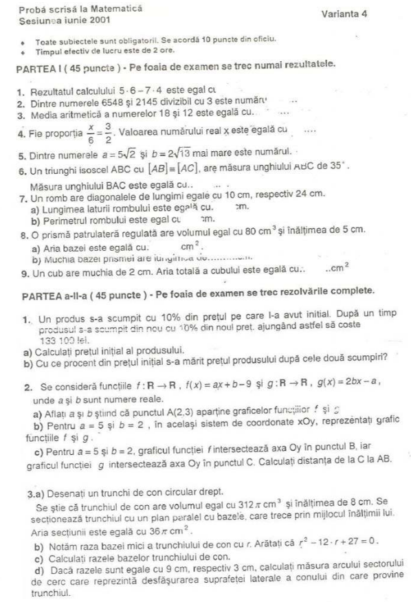
The subjects
The subjects for the Capacitate were the following. We had two hours to solve them:
Translation into English + Solutions
First Part (Partea 1)
- The result of \(5*6-7*4\) is:
...- The obvious answer is \(30-28=2\).
- Between \(6548\) and \(2145\), the number divisible by 3 is
...- The rule is simple: for a number to be divisible by 3 the sum of its digits is divisible by 3, so the answer is: \(2145\). (\(2+1+4+5=12\), \(12\) is divisible by \(3\)).
- To solve this exercise, there’s no need to perform the division.
- The arithmetic mean of the numbers \(18\) and \(12\) is
...- This exercise simply asses if the kid understands the concept of an arithmetic mean, the answer is \(15\).
- Given the proportion \(\frac{x}{6}=\frac{3}{2}\), \(x\) is
...- \(x\) is \(\frac{6*3}{2}=9\).
- Between \(a=5\sqrt{2}\) and \(b=2\sqrt{13}\) which one is bigger ?
- The answer is \(2\sqrt{13}\). Back in school, I had to remember a few radicals to use them as needed. \(\sqrt{13}\) was one of them. I have forgotten them by now. We also had to learn the algorithm to compute any \(\sqrt{}\) as needed.
- An isosceles triangle \(\text{ABC}\) with \([AC]\equiv[AC]\) has the angle \(\measuredangle \text{ABC}=35^{\circ}\), what is \(\measuredangle \text{BAC}=\)
...?- The sum of the angles in a triangle is \(180^{\circ}\), and we know that in an isosceles triangle the two angles \(\measuredangle \text{ABC}\) and \(\measuredangle \text{ACB}\) are equal. So the answer is \(\measuredangle \text{BAC}=180^{\circ}-2*35^{\circ}=110^{\circ}\).
- A rhombus has the diagonals \(10\) and \(24\)?
- What is the length of one of its sides?
- The side is \(\sqrt{(\frac{10}{2})^{2}+(\frac{24}{2})^{2}}=13\)
- What is the perimeter of the rhombus?
- Now that we know one side, we multiply its value by \(4*13=52\).
- What is the length of one of its sides?
- A square prism has it’s volume \(80cm^3\), and the height \(5cm^2\)
- The base surface of the prism is
...- Applying the formula, we get the answer \(16cm^2\)
- The side of the prim’s base is
...- Applying the formula, we get \(4cm^2\)
- The base surface of the prism is
- A cube has one of its sides \(2cm\). The total area of the cube is
...- The answer is \(24cm^2\)
Second Part (Partea 2)
- A specific product had a price increase of 10%. After a while, it got a new 10% price increase, and it now costs \(133100 \text{lei}\).
- What was the initial price of the product?
- \(x\) is the initial price of the product;
- \(a=x+\frac{10x}{100}\) is the price of the product after then first 10 percent increase;
- After the second price increase \(a+\frac{10a}{100}=133100\);
- We compute \(a=133100*\frac{100}{110}=121000\);
- We compute \(x=121000*\frac{100}{110}=110000\).
- What is the total price increase in percentages?
- We need to solve this equation \(110000+110000\frac{x}{100}=133100\);
- We determine the total price increase to be \(\frac{21}{100}=21\)%;
- What was the initial price of the product?
- Considering the following functions \(f : \mathbb{R} \rightarrow \mathbb{R}\), \(f(x)=ax+b-9\) and \(g : \mathbb{R} \rightarrow \mathbb{R}\), \(g(x)=2bx-a\) and \(a,b \in \mathbb{R}\):
- Determine \(a,b\) knowing that \(A(2,3)\) belongs to \(f(x)\) and \(g(x)\);
- If \(A(2,3)\) belongs to the \(f(x)\) and \(g(x)\), then the following is true: \(f(2)=a*2+b-9=3\) and \(g(2)=4b-a=3\).
- After solving the system of equations \(a=5\) and \(b=2\).
- For \(a=5\) and \(b=2\) plot \(f(x)\) and \(g(x)\).
- Substituting the values, we get the functions: \(f(x)=5*x+2-9=5*x-7\) and \(g(x)=4*x-5\)
- To plot them, we need to understand where the functions intersects \(OX\) and \(OY\).
- \(f(0)=-7\) so the \(OY\) axis is intersected by \(f(x)\) at \((0, -7)\);
- \(5x-7=0\), we get \(x=\frac{7}{5}\), so the \(OX\) axis is intersected at \((\frac{7}{5}, 0)\);
- \(g(0)=-5\), so the \(OY\) axis is intersected by \(g(x)\) at \((0, -5)\);
- \(4x-5=0\), we get \(x=\frac{5}{4}\), so the \(OY\) axis is intersected at \((\frac{5}{4}, 0)\);
- We plot
- For \(a=5\) and \(b=2\), \(f\) intersects \(OY\) in \(B\), and \(g\) intersects \(OY\) in \(C\). Compute the distances from \(C\) to \(AB\).
- We know that \(A\) is on \(f(x)\) and so is \(B\). So we can safely assume that the line equation for \(AB\) is the given by \(f(x)\), so \(y-5x+7=0\).
- A student can also compute the line equation from two points \(A\) and \(B\) with the formula: \(\frac{x-x_A}{x_B-x_A}=\frac{y-y_A}{y_B-y_A}\), but it’s a little bit overkill.
- We have to compute the distance from \(C(0,-5)\) to \(y-5x+7=0\) or \(-5x+y+7=0\).
- There’s a formula for that, \(d(ax+by+c, P(x_p, y_p))=\frac{\vert ax_p+by_p+c \vert}{\sqrt{a^2+b^2}}\).
- Substituting the values in the formula \(d=\frac{\vert (-5)*(0) + 1 * (-5) + 7 \vert}{\sqrt{(-5)^2 + 1^2}}=\frac{2}{25+1}=\frac{\sqrt{26}}{13}\)
- Determine \(a,b\) knowing that \(A(2,3)\) belongs to \(f(x)\) and \(g(x)\);
Third Part (Partea 3)
- Plot the Frustum of a Right Circular Cone. The volume is \(312\pi \text{cm}^3\), and it’s height is \(8\text{cm}\). We section the frustum with a plane parallel to its base; this plane is going straight through the middle of its height. The surface of this section is \(36\pi \text{cm}^2\).
- The radius of the smaller base of the frustum is \(r\). Prove that \(r^2 - 12*r + 27=0\).
- The vormula for the Volume is \(V=\frac{1}{3}h\pi (R^2 + r^2 + Rr)\).
- If we substitute the values, we obtain \(R^2+r^2+Rr=117\).
(1) - If the surface of the section is \(S_{s}=36\pi=\pi*{r_s}^2\), the radius of the section is \(r_s=\sqrt{36}=6\).
- But, \(\frac{R+r}{2}=r_s\), so we can say that \(R+r=12\).
(2) - Using
(1)in(2), we obtain \(R^2+r(R+r)=(12-r)^2 + r*12=117\). After a few more steps we prove that \(r^2-12r+27=0\).
- Determine the radiuses of the two bases of the frustum.
- We already know the relationship: \(r^2-12r+27=0\) holds true, so we can compute the radiuses as \(3\) and \(9\).
- If the radiuses are \(9\) and \(3\), compute the sector of the arc, which is the lateral unfolding of the frustum.
- There’s a formula for this \(A_l = \pi G(R+r)\), and \(G=\sqrt{h^2+(R-r)^2}=10\). So \(A_l=120\pi \text{cm}^2\).
The second important exam - Bacalaureat (2005)
Just like Capacitate, Bacalaureat is tailored in a way you can pass it (the minimum requirement is 5/10), but it makes it harder to score 10/10. Again, I couldn’t score 10/10, but 9.90/10 was close.
In Romania, if you opt for a matematica-informatica specialization, you study pieces of everything: some advanced algebra, basic statistics, linear algebra, descriptive geometry, and lots of real analysis.
The syllabus
The high school math syllabus is quite intense, or at least this is how I’ve felt it to be. I had to allocate lots of extra time to grasp the concepts my brilliant teacher constantly threw at me (thanks, Mrs. Georgescu, you were great!).
On the one hand, I am grateful I did a lot of calculus in high school; it helped me with math and physics courses during my University years; on the other hand, I feel that making calculus mandatory for the Baccalaureat punishes too harshly the students who are not mathematically inclined.
The following paragraphs contain a rough translation of the High-School Math Syllabyus (the version from 2017) for the matematica-informatica specialization:
- Sets and Elements of Mathematical Logic (First Year)
- Set of real numbers: algebraic operations with real numbers, ordering of real numbers, absolute value of a real number, approximations by deficiency or by excess, integer part, fractional part of a real number; operations with intervals of real numbers.
- Proposition, predicate, quantifiers
- Basic logical operations (negation, conjunction, disjunction, implication, equivalence), correlated with operations and relations between sets (complement, intersection, union, inclusion, equality); reasoning by reductio ad absurdum.
- Mathematical induction
- Sequences (First Year)
- Ways to define a sequence, bounded sequences, monotonic sequences
- Specific sequences: arithmetic progressions, geometric progressions, the formula for the general term in terms of a given term and ratio, the sum of the first n terms of a progression
- Conditions for n numbers to form an arithmetic or geometric progression
- Functions; Graphical Readings/Representation (First Year)
- Cartesian reference system, Cartesian product; representation through points of a Cartesian product of numerical sets; algebraic conditions for points located in quadrants; lines in the plane of the form \(x=m\), or \(y=m\) with \(m \in \mathbb{R}\).
- Function: definition, examples, examples of correspondences that are not functions, ways to describe a function, graphical readings. Equality of two functions, the image of a set through a function, the graph of a function, restrictions of a function;
- Numerical functions \((F={f:D \rightarrow \mathbb{R}, D \subseteq \mathbb{R}})\); geometric representation of the graph: intersection with the coordinate axes, graphical solutions of equations and inequalities of the form \(f(x)=g(x), (\gt, \lt, \geq, \leq)\); properties of numerical functions introduced through graphical reading: boundedness, monotonicity; other properties: parity/oddity, symmetry of the graph with respect to lines of the form \(x=m\), \(m \in \mathbb{R}\), periodicity;
- Function composition
- First-Degree Function (First Year)
- Definition; graphical representation of the function: \(f:\mathbb{R} \rightarrow \mathbb{R}\), \(f(x)=ax+b\), where \(a, b \in \mathbb{R}\)
- Intersection of the graph with the coordinate axes
- Graphical interpretation of the algebraic properties of the function: monotonicity and the sign of the function; studying monotonicity through the sign of the difference \(f(x_{1})-f(x_{2})\) (or by studying the sign of the ratio: \(\frac{f(x_1)-f(x_2)}{x_{1}-x_{2}})\), \(x_1, x_2 \in \mathbb{R}, x_1 \neq x_2\).
- Inequalities of the form \(ax+b (\gt, \lt, \geq, \leq) 0\) studied on or over intervals of real numbers.
- Systems of first-degree inequalities
- Second-Degree Function (First Year)
- Graphical representation of the function: \(f:\mathbb{R} \rightarrow \mathbb{R}\), \(f(x)=ax^2+bx+c\), \(a,b,c \in \mathbb{R}, a \neq 0\), intersection of the graph with the coordinate axes, equation \(f(x)=0\), symmetry with respect to lines of the form \(x=m\), \(m \in \mathbb{R}\)
- Viète’s relations
- Geometric Interpretation of the Algebraic Properties of the Second-Degree Function (First Year)
- Monotony; studying monotony through the sign of the difference \(f(x_1)-f(x_2)\) or through the rate of increase/decrease: \(\frac{f(x_1)-f(x_2)}{x_1-x_2}\), extreme point, vertex of the parabola;
- Positioning of the parabola relative to the x-axis, the sign of the function, inequalities of the form \(ax^2+bx+c(\gt, \lt, \geq, \leq) 0\), \(a, b, c \in \mathbb{R}, a \neq 0\), on or over intervals of real numbers, geometric interpretation: images of intervals (projections of portions of a parabola onto the y-axis);
- Relative position of a line with respect to a parabola
- Vectors in the Plane (First Year)
- Oriented segment, vectors, collinear vectors
- Vector operations: addition (triangle rule, parallelogram rule), properties of the addition operation; scalar multiplication, properties of scalar multiplication; collinearity condition, decomposition along two non-collinear vectors
- Collinearity, concurrency, parallelism - vector calculus in plane geometry (First Year)
- Position vector of a point
- Position vector of the point that divides a segment in a given ratio, Thales’ theorem (conditions for parallelism)
- Position vector of the centroid of a triangle (concurrency of medians of a triangle)
- Menelaus’ theorem, Ceva’s theorem
- Elements of Trigonometry (First Year)
- Trigonometric circle, definition of trigonometric functions;
- Reduction to the first quadrant; trigonometric formulas
- Applications of Trigonometry and the Scalar Product of Two Vectors in Plane Geometry (First Year)
- Scalar product of two vectors: definition, properties. Applications: cosine theorem, conditions of perpendicularity, solution of right-angled triangles
- Vector and trigonometric applications in geometry: sine theorem, solution of arbitrary triangles
- Calculation of the radius of the inscribed and circumscribed circles in a triangle, calculation of lengths of important segments in a triangle, calculation of areas
- Sets of Numbers (Second Year)
- Real numbers: properties of powers with rational, irrational, and real exponents of a positive non-zero number, rational approximations for real numbers
- \(n\)th root (\(n \in \mathbb{R}\)) of a number, properties of radicals;
- Notion of logarithm, properties of logarithms, calculations with logarithms, logarithmic operation
- Set of complex numbers in algebraic form, conjugate of a complex number, operations with complex numbers. Geometric interpretation of addition and subtraction operations of complex numbers and their multiplication by a real number
- Solving a quadratic equation with real coefficients. Quadratic equations
- Functions and Equations (Second Year)
- Power function with a natural exponent: \(f:\mathbb{R} \rightarrow D\), \(f(x)=x^n\), \(n \in \mathbb{N}\), \(n \geq 2\)
- Radical function: \(f:\mathbb{R} \rightarrow D\), \(f(x)=(x)^{\frac{1}{n}}\), \(n \in \mathbb{N}\), \(n \geq 2\), \(D=[0, \infty)\), \(n\) even or odd;
- Exponential function: \(f:[0, \infty)\), \(f(x)=a^x\), \(a \ge 0\), \(a \neq 1\);
- Logarithmic function: \(f:[0, \infty]\), \(f(x)=log_{a}(x)\), \(a \ge 0\), \(a \neq 1\);
- Injectivity, surjectivity, bijectivity; invertible functions: definition, graphical properties, necessary and sufficient condition for a function to be invertible
- Direct and inverse trigonometric functions
- Counting Methods (Second Year)
- Ordered finite sets. Number of functions \(f:A \rightarrow B\), where \(A, B\) are finite Sets;
- Permutations:
- Number of ordered sets obtained by arranging a finite set with \(n\) elements
- Number of bijective functions \(f:A \rightarrow B\), where \(A,B\) are finite Sets;
- Arrangements
- Number of ordered subsets with k elements, \(k \leq n\), that can be formed with \(n\) elements of a finite Sets;
- Number of injective functions \(f:A \rightarrow B\), where \(A, B\) are finite Sets;
- Combinations
- Number of subsets with k elements, \(0 \leq k \leq n\), of a finite Sets with \(n\) elements. Properties: complementary combinations formula, number of all subsets of a set with \(n\) elements
- Newton’s Binomial
- Financial Mathematics (Second Year)
- Elements of financial calculations: percentages, interest, VAT
- Collection, classification, and processing of statistical data: statistical data, graphical representation of statistical data
- Interpretation of statistical data through position parameters: means, variance, deviations from the mean
- Equally likely random events, operations with events, probability of a compound event composed of equally likely events
- Geometry (Second Year)
- Cartesian coordinate system in the plane, coordinates of a vector in the plane, coordinates of the sum of vectors, coordinates of the product between a vector and a real number, Cartesian coordinates of a point in the plane, distance between two points in the plane
- Equations of a line in the plane determined by a point and a given direction, and equations of a line determined by two distinct points
- Conditions for parallelism, conditions for the perpendicularity of two lines in the plane; calculation of distances and areas
- Matrices and Systems of Linear Equations (Third Year)
- Matrices;
- Matrix operations: addition, multiplication, multiplication of a matrix by a scalar, properties;
- Determinants;
- Systems of Linear Equations;
- Invertible matrices for \(n \leq 4\);
- Matrix equations;
- Linear systems with at most 4 unknowns, Cramer’s systems, matrix rank
- Study of compatibility and solution of systems: Kronecker-Capelli property, Rouchè property, Gaussian method
- Applications: equation of a line determined by two distinct points, area of a triangle, and collinearity of three points in the plane
- Elements of Real Analysis (Third Year)
- Elementary notions about sets of points on the real line: intervals, boundedness, neighborhoods, closed line, symbols ∞ and −∞
- Real functions of a real variable: polynomial function, rational function, power function, radical function, logarithmic function, exponential function, direct and inverse trigonometric functions
- Limit of a sequence using neighborhoods, convergent sequences
- Monotony, boundedness, limits; the squeeze theorem
- Weistrass Property
- The number \(e\)
- Limits in the form \(((1+u_n)^\frac{1}{u_n})\), \(u_n \rightarrow 0\), \(u_n \neq 0\), \(n \in N\);
- Operations with Sequences that have a Limit
- Limits of functions: graphical interpretation of the limit of a function at a point using neighborhoods, one-sided limits
- Calculation of limits for the studied functions; exceptional cases in the calculation of limits of functions
- Asymptotes of the graph of studied functions: vertical asymptotes, oblique asymptotes
- Function Continuity (Third Year)
- Continuity of a function at a point in its domain, continuous functions, graphical interpretation of the continuity of a function, studying continuity at points on the real line for the studied functions, operations with continuous functions
- Darboux’s property, the sign of a function continuous on an interval of real numbers, studying the existence of solutions to equations in \(\mathbb{R}\);
- Differentiability (Third Year)
- Tangent to a curve, derivative of a function at a point, differentiable functions, operations with differentiable functions, calculation of first and second-order derivatives for the studied functions
- Functions differentiable on an interval: extreme points of a function, Fermat’s theorem, Rolle’s theorem, Lagrange’s theorem and their geometric interpretation, the corollary of Lagrange’s theorem regarding the derivative of a function at a point
- The role of the first derivative in the study of functions: monotony of functions, extreme points
- The role of the second derivative in the study of functions: concavity, convexity, inflection points
- L’Hôpital’s rules
- Graphical Representation of Functions (Third Year)
- Graphical representation of functions
- Graphical solution of equations, using the graphical representation of functions to determine the number of solutions to an equation
- Graphical representation of conics (circle, ellipse, hyperbola, parabola)
- Advanced Algebra (Third Year)
- Groups
- Internal composition law (algebraic operation), operation table, stable part
- Group, examples: numerical groups, matrix groups, permutation groups, additive group of residue classes modulo \(n\)
- Subgroup
- Finite group, operation table, order of an element
- Morphism, group isomorphism
- Rings and Fields
- Ring, examples: numerical rings (\(Z, Q, R, C\)), \(Z_{n}\), matrix rings, rings of real functions
- Field, examples: numerical fields (\(Q, R, C\)), p-primary
- Ring and field morphisms
- Polynomial Rings with Coefficients in a Commutative Field (Q, R, C, \(Z_p\), p-primary)
- Algebraic form of a polynomial, polynomial function, operations (addition, multiplication, scalar multiplication)
- Remainder theorem; polynomial division, division by \(X−a\), Horner’s scheme
- Polynomial divisibility, Bézout’s theorem; greatest common divisor and least common multiple of polynomials, factorization of polynomials into irreducible factors
- Roots of polynomials, Viète’s relations
- Solving algebraic equations with coefficients in (\(Z, Q, R, C\)), binomial equations, quadratic equations, reciprocal equations
- Groups
- Real Analysis (Fourth Year)
- Antiderivatives of a function defined on an interval. Indefinite integral of a function, properties of the indefinite integral, linearity. Standard antiderivatives
- Definite Integral
- Subdivisions of an interval \([a,b]\), norm of a subdivision, system of intermediate points, Riemann sums, geometric interpretation. Definition of the integrability of a function on an interval \([a,b]\);
- Properties of the definite integral: linearity, monotony, additivity with respect to the integration interval.
- Leibniz-Newton formula
- Integrability of continuous functions, mean value theorem, geometric interpretation, theorem of the existence of primitives for a continuous function
- Methods of calculating definite integrals: Integration by parts, integration by change of variable.
- Calculation of integrals of the form \(\int_{a}^{b} \frac{P(x)}{Q(x)} dx\), using the method of partial fraction decomposition.
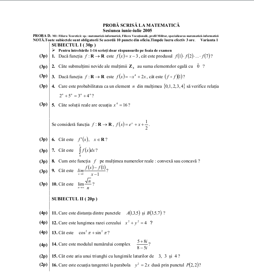
The Exercises
The Bacalaureat exercises I had to solve (in 3 hours) were the following:
Translation into English to Solutions
Subiectul 1
- If \(f:\mathbb{R} \rightarrow \mathbb{R}\) is \(f(x)=x-3\), what is the value of the prouct \(f(1)*f(2)*...*f(7)\)?
- f(3)=0, so the product is itself 0. No need for additional computations.
- How many non-empty subsets of the set \(\mathbb{Z}_{3}\) have a sum of elements equal to 0̂?
- \(\mathbb{Z}_{3}\) refers to the set of integers modulo 3.
- We will have to consider various combinations and check the condition.
- The subsets are \(\{0\}\), \(\{1,2\}\), and \(\mathbb{Z}_{3}\), so the final answer is 3.
- If the function \(f:\mathbb{R} \rightarrow \mathbb{R}\) is \(f(x)=-x^4+2x\) what is the value of \((f \circ f)(1)\) ?
- We start with the definition \((f \circ f)(x)=f(f(x))=-(-x^4+2x)^4 + 2(-x^4+2x)\)
- We substitue \(x=1\), \((f \circ f)(1)=-1+2=1\)
- What is the probability that an element n from the set \(\{0, 1, 2, 3, 4\}\) satisfies the relationship \(2^n + 5^n = 3^n + 4^n\) ?
- The relantionship is satisfied if \(n=0\) or \(n=1\), using the formula for probabilities, the answer is \(P=\frac{2}{5}\).
- How many real solutions does the \(x^4=16\) equation have?
- \((x^4)=(x^2)^2=4\), because \(x \in \mathbb{R}\), the real solutions are \(2\) and \(-2\), so the answer is 2.
Considering the function: \(f:\mathbb{R}\), \(f(x)=e^x+x+\frac{1}{2}\).
- Compute \(f'(x)\).
- We simply compute: \(f'(x)=(e^x+x+\frac{1}{2})' = e^x + 1\)
- Compute \(\int_{0}^{1}f(x)dx\).
- We simply compute: \(\int_{0}^{1}f(x)dx=\int_{0}^{1}(e^x+x+1)dx=(e^x+\frac{x^2}{2}+\frac{x}{2}) \Big\|_0^1=e\).
- How is the function \(f\) over the set of real numbers: convex or concave?
- We differentiate the function twice and check the conditions:
- If \(f''(x) \geq 0\), then the function is convex
- If \(f''(x) \leq 0\), then the function is concave
- We know \(f'(x)=e^x+1\), so we can easily compute \(f''(x)=e^x\).
- It’s a known fact that \(e^x \geq 0\) so the answer is: \(f\) is convex on \(\mathbb{R}\).
- We differentiate the function twice and check the conditions:
- What is the limit: \(\lim_{x \to 1} \frac{f(x)-f(1)}{x-1}\) ?
- Cheesy one. The definition of the derivative in \(a\) is: \(\lim_{x \to a} \frac{f(x)-f(a)}{x-a}\);
- We have to compute \(f'(1)=e^1+1=e+1\). The answer is \(e+1\).
- What is the limit \(\lim_{x \to \infty} \frac{\sqrt{n}}{n}\) ?
- We can do this simple trick: \(\lim_{n \to \infty} \frac{\sqrt{n}}{n}=\lim_{n \to \infty}\frac{\sqrt{n}}{\sqrt{n}*\sqrt{n}}=\frac{1}{\infty}=0\).
Subiectul 2
- What is the distance between the two points: \(A(1,3,5)\) and \(B(3,5,7)\)?
- We compute the distance: \(d=\sqrt{(3-1)^2+(5-3)^2+(7-5)^2}=\sqrt{3*2^2}=2*\sqrt{3}\)
- What is the radius of the circle: \(x^2+y^2=4\) ?
- The answer is \(r=2\) (fundamental equation of the circle)
- What is \(cos^2\pi + sin^2\pi\) ?
- The answer is 1, as per the fundamental: \(sin^2x+cos^2x=1\).
- What is the modulus of the complex number \(z=\frac{5+8*i}{8-5*i}\)?
- We need to compute: \(\vert z \vert\).
- If \(z=a+b*i\), then \(\vert z \vert=\sqrt{a^2+b^2}\)
- We need to reduce our \(z\) to a form were it’s easy to identity \(a\) and \(b\)
- In this regard, we can write \(z=\frac{(5+8*i)(8+5*i)}{(8-5*i)(8+5*i)}\)
- After doing all the computations: \(z=i\), so \(\vert z \vert=1\)
- What is the area of a triangle with its sides: \(3\), \(3\) and \(4\) ?
- The elegant way of doing it is to apply Heron’s theorem: \(A=\sqrt{p(p-a)(p-b)(p-c)}\), where \(p=\frac{a+b+c}{2}\).
- The answer is \(A=\sqrt{5*2*2*1}=2*\sqrt{5}\).
- What is the equation of the tangent line to the parabola \(y^2 = 2x\) passing through the point \(P(2, 2)\)?
- Applying the equation, we get to the form: \(2*y=x+2\).
Subiectul 3
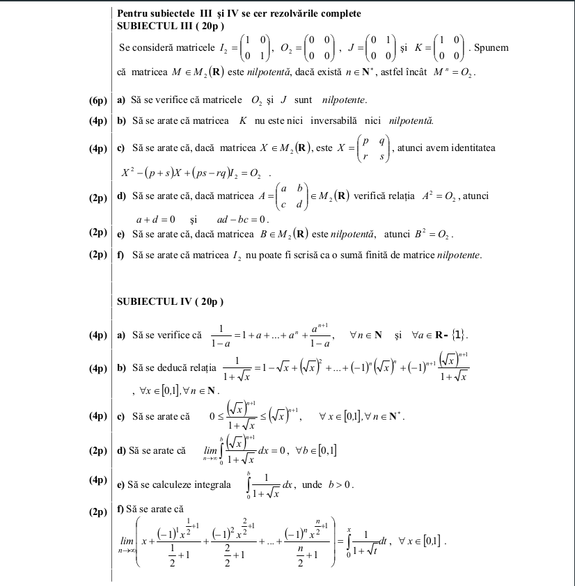
Considering the matrices: \(I=\begin{pmatrix} 1 & 0 \\ 0 & 1 \end{pmatrix}\), \(O_{2}=\begin{pmatrix} 0 & 0 \\ 0 & 0 \end{pmatrix}\), \(J=\begin{pmatrix} 0 & 1 \\ 0 & 0 \end{pmatrix}\), \(K=\begin{pmatrix} 1 & 0 \\ 0 & 0 \end{pmatrix}\), a matrix \(M \in M_{2}(\mathbb{R})\) is nilpotent, if there is \(n \in \mathbb{N}^{*}\), so that \(M^n=O_2\).
- Prove that \(O_2\) and \(J\) are nilpotent
- \(O_2^n=O_2\), \(∀ n \in \mathbb{N}^{*}\), so we can pick an arbitrary \(n\), and the nilpotency condition is satisfied.
- For \(J\) we just compute \(J^2\), and it becomes evident that the nilpotency condition is satisfied for \(n=2\).
- Show that the \(K\) matrix is neither inversible nor nilpotent.
- For a matrix to be invertible, \(det(A) \neq 0\), but \(det(K)=0\), so \(K\) is not invertible;
- We can prove \(K^n=K\), \(∀ n \in \mathbb{N}^{*}\), but \(K \neq O_2\), so \(K\) is not nilpotent;
- Prove that \(X \in M_2(\mathbb{R})\), \(X=\begin{pmatrix} p & q \\ r & s \end{pmatrix}\), satisfies the identity: \(X^2 - (p+s)X + (ps-rq)I_2=O_2\).
- First step is to compute \(X^2\).
- In this regard: \(X^2=\begin{pmatrix} p^2 + qr & pq + qs \\ rp + rs & s^2 + qr\end{pmatrix}\);
- The second step is to compute \((p+s)X=\begin{pmatrix} (p+s)p & (p+s)q \\ (p+s)r & (p+s)s \end{pmatrix}\);
- And lastly, we need to compute \((ps-rq)I_2=\begin{pmatrix} (ps-qr) & 0 \\ 0 & (ps-qr)\end{pmatrix}\);
- Putting it all together, the relationship is verified: \(X^2 - (p+s)X + (ps-rq)I_2=O_2\).
- Prove that if \(A=\begin{pmatrix} a & b \\ c & d \end{pmatrix} \in M_2(\mathbb{R})\) checks the relationship \(A^2=O_2\), then \(a+d=0\) and \(ad-bc=0\).
- If we look closely: \(a+d\) is the trace of A \(tr(A)\);
- Again, \(ad-bc\) is actually the determinant of \(A\);
- Now, if \(A=O_2\), then both the trace and determinant are \(0\);
- If \(A \neq O_2\), the relationship proved at the previous point becomes \(A^2 - tr(A)*A + det(A)*I_2=O_2\).
- But \(A^2=O_2\), so the relationship becomes: \(tr(A)*A=det(A)*I_2\).
- If we multiply each side of the previous equality with \(A\), and remember that \(A^2=O_2\), we get to \(det(A)*A=0\). But because we’ve decided that \(A \neq O_2\), we know that \(det(A)=0\), then \(ad-bc=0\).
- Given that \(det(A)=0\) and \(A^2=O_2\), then \(\underbrace{A^2}_{0}-tr(A)*A + \underbrace{det(A)*I_2}_{0}=O_2\), then \(tr(A)*A=O_2\), then \(tr(A)=0\), then \(a+d=0\).
- Prove that if \(B \in M_2({\mathbb{R}})\) is nilpotent, then \(B^2=O_2\).
- If \(B\) is nilpotent, then a number \(n \in \mathbb{N}^{*}\) exists, such that \(B^{n}=O_2\);
- If \(B^n=O_2\), we can say the same about \((B^n)^2=O_2\).
- Given the previously proved relationship, we also know that \(tr(B^n)\) and \(det(B^n)\) are \(0\).
- As a known identity, \(det(M * N)=det(M)*det(N)\), \(∀ M, N \in M_m(\mathbb{C})\), so inductively we keep in mind the fact that \(det(M^k)=det(M)^k\);
- Now, let’s get back and find our \(n\). We introduce \(n_0\), \(n_0 \in \mathbb{N}^{*}\), the first \(n\) that satisfies the condition;
- We know that \(det(B^{n_0})=0\), and so \(det(B)^{n_0}=0\). The only possible way to satisfy that is if \(det(B)=0\).
- So the relationship proved at
3.becomes \(B^2-tr(B)*B=0\). If we multiply each side with \(B^{n_0-2}\), we get \(B^n_0-tr(B)*B^{n_0-1}=O_2\). - But we already said that \(B^{n_0}=O_2\), this means that \(tr(B)*B^{n_0-1}=0\) so \(tr(B)=0\)
- At this point, all the conditions are met, and we can safely say that \(B^2=O_2\);
- Prove that \(I_2\) cannot be written as an infinite sum of nilpotent matrices;
- Ad absurdum, we say that \(I_2=\sum_{k=1}^{n}*A_k\), where \(A_k\) is nilpotent and \(k \in [1, \infty)\).
- Because \(A_k\) is nilpotent, then \(A_k^2=O_2\) and \(tr(A)=0\) (see
4.); - Through induction we can prove that \(tr(\sum_{k=1}^{\infty}A_k)=\sum_{k=1}^{\infty} tr(A_k)\);
- If our supposition that \(I_2=\sum_{k=1}^{n}*A_k\) was correct, then \(tr(\sum_{k=1}^{\infty}A_k)=0\). But that would be incorrect because \(tr(I_2)=2\), so our supposition was proved to be false.
Subiectul 4
- Verify that \(\frac{1}{1-a}=1+a+...+a^n+\frac{a^{n+1}}{1-a}\), \(∀ n \in \mathbb{N}\) and \(∀ a \in \mathbb{R}-\{1\}\).
- We observe that \(1, a, a^2, a^3, ... , a^n\) are the first \(n+1\) terms of a geometric progression that starts with \(1\) and has \(a\) as the ratio.
- Using the formula, \(1+a+a^2+...+a^n=\frac{1-a^{n+1}}{1-a}=\frac{1}{1-a} - \frac{a^{n+1}}{1-a}\).
- Thus, \(\frac{1}{1-a}=1+a+...+a^n+\frac{a^{n+1}}{1-a}\)
- Prove the relationship \(\frac{1}{1+\sqrt{x}}=1-\sqrt{x}+(\sqrt{x})^2+...+(-1)^n(\sqrt{x})^n+(-1)^{n+1}\frac{(\sqrt{x})^{n+1}}{1+\sqrt{x}}\), \(∀ x \in [0,1], ∀ n \in \mathbb{N}\).
- Just by looking at
1.and2.we see a similar pattern. - The solution is to substitute \(a=-\sqrt{x}\), and the required relationship is proven.
- Just by looking at
- Prove that \(0 \leq \frac{(\sqrt{x})^{n+1}}{1+\sqrt{x}} \leq (\sqrt{x})^{n+1}\), \(∀ x \in [0,1], ∀ n \in \mathbb{N}\).
- We prove the two equalities one by one.
- We know that \((\sqrt{x})^{n+1} \geq 0\);
- We also know that \(\sqrt{x}+1 \geq 0\).
- We can then conclude that the ratio is also positive \(\frac{(\sqrt{x})^1} \geq 0\).
- \(\sqrt{x}\) is also an increasing function for \(x\) in our domain, so that the second is true;
- Prove that \(\lim_{n \rightarrow \infty}\int_{0}^{b}\frac{(\sqrt{x})^{n+1}}{\sqrt{x}+1}dx=0\), \(∀ \in [0,1]\).
- We make use of the previously proven inequality so we can squeeze our integral like this: \(0 \leq \int_{0}^{b}\frac{(\sqrt{x})^{n+1}}{\sqrt{x}+1}dx \leq \int_{0}^{b}(\sqrt{x})^{n+1}dx\)
- We determine \(\int_{0}^{b} (\sqrt{x})^{n+1}dx=\int_{0}^{b}x^{\frac{n+1}{2}}dx=\frac{x^{\frac{n+1}{2}+1}}{\frac{n+3}{2}}\Big\|_0^b=\frac{2}{n+3}*b^{\frac{n+3}{2}}\)
- We now use this in the limit: \(\lim_{n \rightarrow \infty}\int_{0}^{b} (\sqrt{x})^{n+1}dx=\lim_{n \rightarrow \infty} \frac{2}{n+3}*b^{\frac{n+3}{2}}\)
- We can write the limit \(\lim_{n \rightarrow \infty} \frac{2}{n+3}*b^{\frac{n+3}{2}}=(\lim_{n \rightarrow \infty}\frac{2}{n+3})*(lim_{n \rightarrow \infty}b^{\frac{n+3}{2}}) = 0 * k = 0\), where \(k \in \{0,1\}\).
- At this point, it is squeezed between two \(0\)s, so we’ve proven the limit to be 0;
- Compute the following integral: \(\int_{0}^{b}\frac{1}{1+\sqrt{x}}dx\), \(b > 0\).
- We the following substitution: \(y=1+\sqrt{x}\), so that \((1+\sqrt x)dx=dy\), or \(2*\sqrt{x}dy=dx\), or \(dx=(2y-1)dy\).
- If \(x=0\), then \(y=1\)
- If \(x=b\), then \(y=1+\sqrt{b}\)
- So \(\int_{0}^{b}\frac{1}{1+\sqrt{x}}dx = 2 * \int_{1}^{1+\sqrt{b}} \frac{y-1}{y}dy=2*\int_{0}^{1+\sqrt{b}}dy - \int_{1}^{1+\sqrt{b}}\frac{1}{y}dy\);
- After every computation is done, the result is: \(\int_{0}^{b}\frac{1}{1+\sqrt{x}}dx=2*(\sqrt{b}-ln(1+\sqrt{b}))\)
- Prove that \(\lim_{n \rightarrow \infty} (x + \frac{(-1)^1x^{(\frac{1}{2}+1)}}{\frac{1}{2}+1} + \frac{(-1)^2x^{(\frac{2}{2}+1)}}{\frac{2}{2}+1} + ... + \frac{(-1)^nx^{(\frac{n}{2}+1)}}{\frac{n}{2}+1})=\int_{0}^{x}\frac{1}{1+\sqrt{t}}dt\), \(∀ x \in [0,1]\).
- We start with the integral. We’ve already worked on it at
2.. - We change to \(t\), \(\int_{0}^{x}\frac{1}{1+\sqrt{t}}dt=\int_{0}^{x}(1-\sqrt{t}+(\sqrt{t})^2+...+(-1)^n(\sqrt{t})^n + (-1)^{n+1}\frac{(\sqrt{t})^{n+1}}{1+\sqrt{t}})dt\).
- This also can be written as a sum of two integrals: \(\int_{0}^{x}\frac{1}{1+\sqrt{t}}dt=\int_{0}^{x}(1-\sqrt{t}+(\sqrt{t})^2+...+(-1)^n(\sqrt{t})^n)dt+\int_{0}^{x}((-1)^{n+1}\frac{(\sqrt{t})^{n+1}}{1+\sqrt{t}})dt\)
- The relationship then becomes: \(\int_{0}^{x}\frac{1}{1+\sqrt{t}}dt=(x+\frac{(-1)*x^{\frac{1}{2}+1}}{\frac{1}{2}+1}+...+\frac{(-1)^{n}*x^{\frac{n}{2}+1}}{\frac{n}{2}+1})+(-1)^{n+1}\int_{0}^{x}\frac{(\sqrt{t})^{n+1}}{1+\sqrt{t}}dt\)
- We apply the limit on the last relationship: \(lim_{n \rightarrow \infty}\int_{0}^{x}\frac{1}{1+\sqrt{t}}dt=\lim_{n \rightarrow \infty}(x+\frac{(-1)*x^{\frac{1}{2}+1}}{\frac{1}{2}+1}+...+\frac{(-1)^{n}*x^{\frac{n}{2}+1}}{\frac{n}{2}+1})+\underbrace{lim_{n \rightarrow \infty}((-1)^{n+1}\int_{0}^{x}\frac{(\sqrt{t})^{n+1}}{1+\sqrt{t}})dt}_{0}\)
- Our relationship is proved.
- We start with the integral. We’ve already worked on it at
The third exam - Admiterea la Politehnica (2005)
A good Baccalaureat grade was insufficient to get admitted to the UPB. You had to pass an additional admission exam. This one was a little harder than the Bacaluareat, but not impossible. The catch was not to make any mistakes. Any wrong answer could’ve been fatal.
On day one, you had to pass an exam composed of Algebra + Real Analysis, and on the second day, you had a Physics Exam where you were free to pick two areas. I’ve decided to pick Classical Mechanics and Thermodynamics.
In this section, I will cover only the Math part.
The subjects
You had two hours to solve the following:

The translations + solutions
- Determine \(m \in \mathbb{R}\) so that \(f:\mathbb{R} \rightarrow \mathbb{R}\), \(f(x)=\begin{cases}x^2-2x+m &, m \leq 1 \\ e^x-e &, x \gt 1\end{cases}\) to be continuos on \(\mathbb{R}\):
- Both \(x^2-2x+m\) and \(e^x-e\) are elementary functions, so we can say they are continuous on their intervals;
- So we need to see what’s happening when \(x=1\);
- We need to check the limits (from both sides) for \(f(x)\);
- The limit from the left: \(\lim_{x \rightarrow 1}f(x)=f(1)=m-1\)
- The limit from the right: \(\lim_{1 \leftarrow x}f(x)=f(1)=0\)
- The conclusion is simple \(m-1=0\), so \(m=1\)
- Solve the following inequation: \(\sqrt{x} \lt 1\).
- This is a simple one: \(x \in [0, 1)\)
- What’s the value for the following expression: \(E=\frac{1}{\sqrt{2}+\sqrt{3}}+\frac{1}{\sqrt{3}-\sqrt{2}}\)?
- The expression is equivalent to: \(E=\frac{\sqrt{3}-\sqrt{2}}{3-2}+\frac{\sqrt{3}+\sqrt{2}}{3-2}=2\sqrt{3}\)
- Compute the limit \(\lim_{n \rightarrow \infty}(\sqrt{n^2+n}-\sqrt{n^2+1})\).
- The limit is equivalent to: \(\lim_{n \rightarrow \infty}(\frac{n^2+n-n^2-1}{\sqrt{n^2+n}+\sqrt{n^2+1}})\);
- Then we do the following trick: \(\lim_{n \rightarrow \infty}(\frac{n(1-\frac{1}{n})}{n*(\sqrt{1+\frac{1}{n}}+\sqrt{1+\frac{1}{n^2}})})\)
- But \(\frac{1}{n} \rightarrow 0\) and \(\frac{1}{n^2} \rightarrow 0\) when \(n \rightarrow \infty\), so if we take that into the account the answer is \(\frac{1}{2}\).
- Given the equation \(x^2-ax+4=0\), \(a \in \mathbb{R}\). \(x_1, x_2\) solutions to the equation verify \(x_1 + x_2=5\) if:
- a) \(a=4\); b) \(a=0\); c) \(x_1=x_2\); d) \(a <0\); e) \(a=5\); f) \(x1, x2 \not\in \mathbb{R}\)
- Well, \(x_1+x_2=a\), then the correct answer is \(a=5\)
- The solutions for the equation \(9^x-4*3^x+3=0\) are?
- We consider \(y=3^x\), so the equation in \(y\) becomes: \(y^2-4y+3=0\);
- Then, \(y^2-3y-y+3=0\), or \((y-3)(y-1)=0\), the solutions are \(y_1=3\) and \(y_2=1\);
- This means \(3^x=3^1\), the exponential is injective, we can safely say \(x_1=1\) one of the two solutions;
- It also means \(3^x=3^0\), so \(x_2=0\) is the other solution
- Determine \(m, n \in \mathbb{R}\) so that the equation: \(x^4+3x^3+mx^2+nx-10=0\) to admit the solution \(x_1=i\):
- We substitute \(x=i\), so the equation becomes: \(i^4+3i^3+mi^2+ni-10=0\)
- We obtain \((-m-9) + i(n-3)=0\), this is a complex number.
- \((-m-9)\) needs to be \(0\), \(n-3\) needs to be \(0\)
- The answer is \(m=-9\) and \(n=3\)
- Compute the 10th term of the arithmetic progression starting with \(a_1=5\), with the \(r=2\).
- Using the formula we get: \(a_10=a_1+(10-1)*r=23\)
- Compute \(\int_{0}^{1}\frac{x^2}{x^3+1}dx\)
- We write as: \(\int_{0}^{1}\frac{x^2}{x^3+1}dx=\frac{1}{3}\int_{0}^{1}\frac{3*x^2}{x^3+1}dx\)
- We observe the integral can further be written as: \(\frac{1}{3}\int_{0}^{1}\frac{(x^3+1)'}{x^3+1}dx\)
- This is a known form, the answer is: \(\frac{1}{3}ln(2)\)
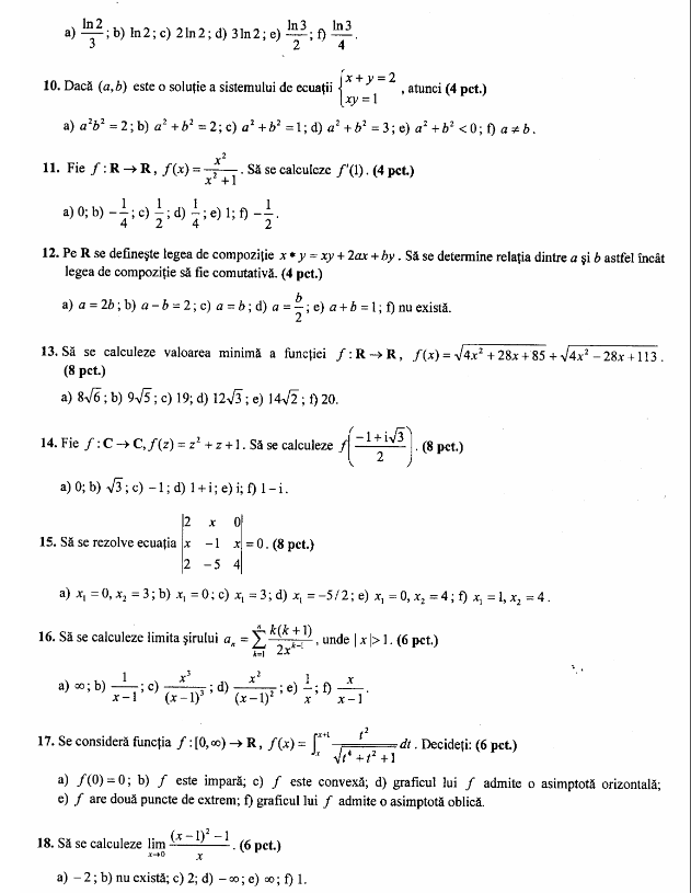
- If \((a,b)\) are a solution for the following system of equations: \(\begin{cases} x+y=2 \\ xy=1\end{cases}\), then:
- a) \(a^2b^2=2\); b) \(a^2+b^2=2\); c) \(a^2+b^2=1\); d) \(a^2+b^2=3\); e) \(a^2 + b^2 < 0\); f) \(a \neq b\)
- We simply solve the system, we see that \(a=1\), and \(b=1\), so the answer is \(a^2+b^2=1\)
- Given \(f:\mathbb{R} \rightarrow \mathbb{R}\), \(f(x)=\frac{x^2}{x^2+1}\). Compute \(f'(1)\):
- We know \(f'(x)=\frac{2x(x^2+1)-x^2*2x}{(x^2+1)^2}\)
- We compute \(f'(1)=\frac{1}{2}\)
- The following composition rule is defined on \(\mathbb{R}\): \(x * y = xy+2ax+by\). Determine the relationship between \(a\) and \(b\) so that the rule is commutative.
- If the rule is commutative, then: \(xy+2ax+by=yx+2ay+bx\)
- After a few more steps: \(2a(x-y)-b(x-y)=0\), or \((x-y)(2a-b)=0\).
- The answer is: \(2a=b\) almost 20 years ago
- What’s the minimum of the following function: \(f:\mathbb{R} \rightarrow \mathbb{R}\), \(f(x)=\sqrt{4x^2+28x+85}+\sqrt{4x^2-28x+113}\)?
- This is pure grind, nothing exciting; the eventual answer will be: \(14\sqrt{2}\).
- Given \(f:\mathbb{C} \rightarrow \mathbb{C}\), \(f(z)=z^2+z+1\), compute \(f(\frac{-1+i\sqrt{3}}{2})\)
- We compute: \(f(\frac{-1+i\sqrt{3}}{2})=\frac{1-3-2*i\sqrt{3}}{4}+\frac{-2+2i\sqrt{3}}{4} + \frac{4}{4}\)
- The final answer is 0;
- Solve the following equation: \(det(\begin{pmatrix} 2 & x & 0 \\ x & -1 & x \\ 2 & -5 & -4\end{pmatrix})=0\)
- Computing the determinant, \(det=x^2-5x+4=0\), \(x=1\) or \(x=4\).
- Compute the limit of \(a_n=\sum_{k=1}^{n}(\frac{k(k+1)}{2x^{k-1}})\), where \(\vert x \vert > 1\)
- After all the grind the result is: \(\frac{x^3}{(x-1)^3}\)
- Given the function: \(f:[0, \infty)\), \(f(x)=\int_{x}^{x+1}\frac{t^2}{\sqrt{t^4+t^2+1}}dt\). Decide if:
- a) f(0) = 0; b) f is odd; c) f is convex; d) f admits a horizontal asymptote; e) f has 2 extreme points f) f admits one oblique asymptote
- We start checking for the following conditions:
- \(f(0)\) is false, f(x) is strictly \(>0\);
- \(f(x)\) cannot be odd, given its domain;
- so both a) and b) are false;
- We differentiate: \(f'(x)=\frac{(x+1)^2}{\sqrt{(x+1)^4 + (x+1)^2 + 1}} - \frac{x^2}{\sqrt{x^4+x^2+1}}=0\)
- After some grind, I am too lazy to write in Latex, we find out that there are no extreme points and and it doesn’t admit any horizontal asymptote
- The final result: \(f''(x)>0\) the the function is convex;
- Compute: \(\lim_{x \rightarrow 0}\frac{(x-1)^2-1}{x}\).
- After applying L’Hopital the result is: \(-2\)
Conclusions
Looking back at everything that was thrown at me 20 years ago, I have a few observations:
- Most of the exercises lack imagination and are either purely theoretical, like the one with matrices from the Bacalaureat or extremely grindy;
- The exams were not complex, but you had to get perfect scores under difficult time constraints;
- The system works, but it lacks any direction.
- In a follow-up article, I plan to select some Olympiad questions I have had to solve through the years. Those are much more interesting and imaginative.
That’s it. How were your exams?
Comments