A tale of Java Hash Tables

Note(s)

• The intended audience for this article is undergrad students who already have a good grasp of Java, or seasoned Java developers who would like to explore an in-depth analysis of various hash table implementations that use Open Addressing.
• The reader should be familiar with Java generics, collections, basic data structures, hash functions, and bitwise operations.

Table of contents

• Introduction
• Separate Chaining, or how HashMap<K,V> works internally
• Open Addressing
  • LProbMap<K, V>
    • Inserting an entry
    • Retrieving an entry
    • Deleting an entry
    • Resizing and rehashing
  • LProbSOAMap<K,V>
  • PerturbMap<K, V>
  • LProbBinsMap<K,V>
  • LProbRadarMap<K, V>
  • RobinHoodMap<K, V>
• Benchmarks
  • RandomStringsReads
  • SequencedStringsReads
  • AlphaNumericCodesReads
• The results
• The results (2)
• Wrapping up
• Discussion

Introduction

In Java, the main hash table implementation, HashMap<K,V>, uses the classical Separate Chaining technique (with critical optimizations that reduce read times in case of collisions).

But, as described here, the decision to use Separate Chaining vs. Open Addressing is not unanimously accepted by programming languages designers. For example, in python, ruby, and rust, the standard hash tables are implemented using Open Addressing, while Java, go, C#, C++ are all more conservatory and use Separate Chaining.

Programming Language	Hash table algorithm	Source(s)
Python	Open Addressing	dictobject.c
Ruby	Open Addressing	st.c
Rust	Open Addressing	map.rs
Java	Separate Chaining	HashMap.java
Go	Separate Chaining	maphash.go
C#	Separate Chaining	Dictionary.cs
C++	Separate Chaining	hashtable.h

There are, of course, lovely hash table implementations that sit outside the standard libraries. So, if you are looking for a good read, check out the Facebook (or should I say Meta) Engineering Blog discussing their super-fast & efficient F14 implementation.

In this article, we will discuss how to implement hash tables in Java, using Open Addressing and then benchmark them against the reference HashMap<K,V> implementation that uses Separate Chaining.

I’ve decided to stay away from Hopscotch, although I did get inspired by it. In regards to Cuckoo Hashing, you can find a “draft” implementation in the code repo.

I’ve also skipped Quadratic probing because I consider python’s approach smarter.

My implementations will be entirely academic, and I am sure a person with more experience optimizing Java code manually will do a better job than me.

Also, given the complex nature of benchmarking Java code, please feel free to comment on the results. I’ve used jmh, but I am more than happy to explore other alternatives.

For the moment, we are going to implement five six Map<K,V> and benchmark their (get()) speed against HashMap<K,V>:

Java Class	Source	Description
LProbMap<K, V>	src	A classic Open Addressing implementation that uses Linear Probing
LProbSOAMap<K,V>	src	This a LProbMap<K,V> alternative implementation with a different memory layout than the original implementation. This was proposed by dzaima on github. Because it’s a cool approach I’ve decided to include it in the article.
LProbBinsMap<K,V>	src	An “almost” classic Open Addressing implementation inspired by ruby’s hash table.
LProbRadarMap<K, V>	src	An Open Addressing implementation that uses a separate vector (radar) to determine where to search for items. It uses the same idea as Hopscotch Hashing
PerturbMap<K, V>	src	An Open Addressing implementation that uses the python’s perturbator algorithm instead of linear probing
RobinHoodMap<K, V>	src	An Open Addressing implementation that uses linear probing with Robin Hood Hashing

The code is available in the following repo:

git clone git@github.com:nomemory/open-addressing-java-maps.git

Before jumping directly to the implementation, I recommend you to read my previous article on the subject. Even if the code is in C, I recommend refreshing a few theoretical insights (e.g., hash functions).

Separate Chaining, or how HashMap<K,V> works internally

As I’ve previously stated, HashMap<K,V> is implemented using a typical Separate Chaining technique. If you jump straight into reading the source code, things can be a little confusing, especially if you don’t know what you are looking for. But once you understand the main concepts, everything becomes much clearer.

Even if this is not the purpose of this article, I believe it’s always a good idea to understand how HashMap<K,V> works. Many (Java) interviewers love to ask this question.

If you already understand how HashMap<K,V> works, you can skip directly to the next section. If you don’t, and you are curious about it, please read the following paragraphs.

The HashMap<K,V> class contains an array of Node<K,V>. For simplicity and inertia, we are going to call this array table:

// The table, initialized on first use, and resized as necessary. 
// When allocated, length is always a power of two. 
transient Node<K,V>[] table;

The table is the most important structure from the class; it’s the place where we store our data.

Node<K,V> class has the following composition:

static class Node<K,V> implements Map.Entry<K,V> {
        final int hash;
        final K key;
        V value;
        Node<K,V> next;

        // getters and setters + other goodies       
}

As you rightfully observed, Node<K,V> is used to implement a “linked” (or chained) data structure. The next attribute references the next Node in the chain.

In this regard, think of the Node<K,V>[] table as an array of linked data structures. For simplicity, let’s suppose those chained structures are linked lists.

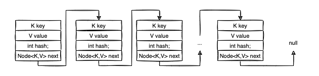
To make things more transparent, let’s analyze the following example. We define a HashMap<String, String>, where keys K are European capital cities (String), while the values V are the corresponding country names (String).

Before doing any insert, there will be one empty table with the initial capacity set to: DEFAULT_INITIAL_CAPACITY=1<<4 (by the magic of bitwise operators, 1<<4==16). The choice of using a power of two is not accidental, we will see shortly why.

Now let’s see what happens when we want to insert the first <String, String> entries: <"Paris", "France">, <"Sofia", "Bulgaria">, <"Madrid", "Spain"> and <"Bucharest", "Romania">.

The put(K key, V value) method is called first, eventually dispatching the call to putVal(...).

public V put(K key, V value) {
    return putVal(hash(key), key, value, false, true);
}

But, before putVal(...) gets called, we need to compute hash(key).

static final int hash(Object key) {
    int h;
    return (key == null) ? 0 : (h = key.hashCode()) ^ (h >>> 16);
}

HashMap<K,V> accepts null keys, so by convention, hash(null) is always 0.

If the key is not null, we shift and xor the hashCode() of the key and return the value.

The reason for doing that extra bit operation is to improve the diffusion of the hashCode() by considering the higher-order bits. If you want to understand more of this magic, please read my previous article: Implementing Hash Tables in C/Hash functions.

If we were to apply the hash method to our input ("Paris", "Sofia", "Madrid", "Bucharest"), we’d obtain the following values:

static final int hash(Object key) {
    int h;
    return (key == null) ? 0 : (h = key.hashCode()) ^ (h >>> 16);
}
public static void main(String[] args) {
    System.out.println(hash("Paris"));      // 76885502
    System.out.println(hash("Sofia"));      // 80061639
    System.out.println(hash("Madrid"));     // -1997818570
    System.out.println(hash("Bucharest"));  // -543452922
}

The next step is to look at the putVal(...) method and see what it does:

final V putVal(int hash, K key, V value, boolean onlyIfAbsent,
                boolean evict) {
    Node<K,V>[] tab; 
    Node<K,V> p; 
    int n, i;
    // If the table is empty we simply allocate space for it
    if ((tab = table) == null || (n = tab.length) == 0)
        n = (tab = resize()).length;
    // Based on the hash we identify an empty slot in the table
    if ((p = tab[i = (n - 1) & hash]) == null) {
        // The slot in the tab is empty so we introduce the <key, value> pair here
        tab[i] = newNode(hash, key, value, null);
    }
    else {
       // The slot is not empty, a collision happened
       // We append the item to the tab
    }
    // More code here
    return null;
}

tab[i = (n - 1) & hash]), where n=table.length, looks like magic, but it’s not.

Because n is a power of two we can use (n-1) & hash to “project” the values from the interval [Integer.MIN_VALUE, Integer.MAX_VALUE] to the table indices: {0, 1, .., n-1}.

It’s a simple trick that works on the power of twos, helping us avoid % (modulo), which is a slow operation.

For our values:

int n = 1<<4;

System.out.println("Paris");
System.out.println(hash("Paris"));          // hash = 76885502
System.out.println((n-1) & hash("Paris"));  // index = 14

System.out.println("Sofia");
System.out.println(hash("Sofia"));          // hash = 80061639
System.out.println((n-1) & hash("Sofia"));  // index = 7

System.out.println("Madrid");
System.out.println(hash("Madrid"));         // hash = -1997818570
System.out.println((n-1) & hash("Madrid")); // index = 6

System.out.println("Bucharest");
System.out.println(hash("Bucharest"));          // hash = -543452922
System.out.println((n-1) & hash("Bucharest"));  // index = 6

So now we can visualize what is happening when we try to insert the entries into the HashMap<K,V>:

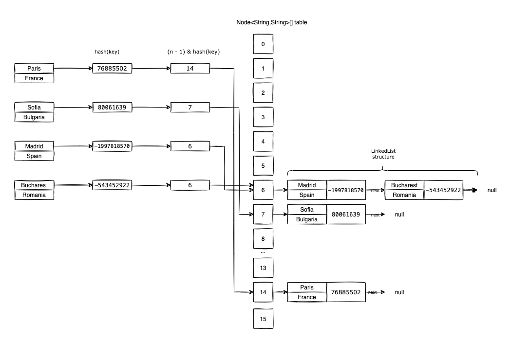
1. The first entry to insert is <"Paris", "France">.
   • We compute hash("Paris")=76885502.
   • We create a new Node<String, String> with hash=76885502, key=Paris, value=France and next=null.
   • Based on the hash we identify the bucket from the table where we are going to insert the entry.
   • Because (16-1) & 76885502 = 14, we insert the newly created node at position table[14].
2. The second entry to insert is <"Sofia", "Bulgaria">.
   • We compute hash("Sofia")=80061639.
   • We create a new Node<String, String> with hash=80061639, key=Sofia, value=Bulgaria and next=null.
   • Based on the hash we identify the bucket from the table where we are going to insert the entry.
   • Because (16-1) & 80061639 = 7, we insert the newly created node at position table[7].
3. The third entry to insert is <Madrid, Spain>.
   • We compute the hash("Madrid")=-1997818570.
   • We create a new Node<String, String> with hash=-1997818570, key=Madrid, value=Spain and next=null.
   • Based on the hash we identify the bucket from the table where we are going to insert the entry.
   • Because (16-1) & (-1997818570) = 6, we insert the newly created node at position table[6].
4. The fourth and last entry to insert is <Bucharest, Romania>.
   • We compute the hash("Bucharest")=-543452922.
   • We create a new Node<String, String> with hash=-543452922, key=Bucharest, value=Romania and next=null.
   • Based on the hash we identify the bucket from the table where we are going to insert the entry.
   • Because (16-1) & (-543452922) = 6, we want to insert our node to table[6].
     • But the position table[6] is already occupied!! This is called a hash collision.
     • The solution is to append our newly created node to the last node from the chain (we use next to point to our newly created node).

Now retrieving an element by its key is simple; we have to follow the same trail as the insertions.

Let’s imagine for example we want to get("Bucharest"):

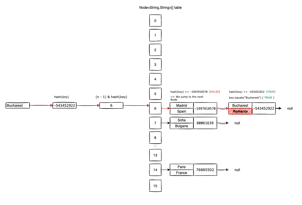
First, we compute the hash("Bucharest")=-543452922 and the possible index where we might find the item in the table, 6 = (16-1) & (-543452922).

At position table[6], there seems to be an item already. But we don’t know for sure if it’s the item we are looking for or another item we’ve collided with when we perform the insertions.

In this regard we compare hash("Bucharest") with table[6].hash. In our case, the hash values are not equal, so we jump to the next item in the chain: table[6].next.

We do the hash comparison again hash("Bucharest)==table[6].next.hash, and this time it’s true.

To be 100% sure we get (retrieving) the correct value we do a final comparison "Bucharest".equals(table[6].next.key). If the two keys are equal, we’ve found the correct value. If not, we continue the two comparisons until we reach the end of the chain table[6].next ... .next.

There’s a slight chance of having two distinct Strings with the same hash(..) value. That’s why we perform the additional comparison using equals(...) - to make sure we eliminate this possibility.

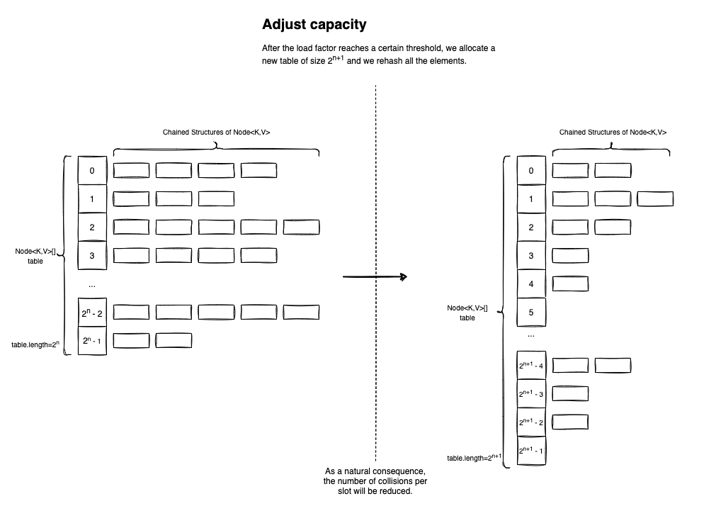
To make things more efficient, the HashMap<K,V> performs two types of optimizations while we insert (lots of) elements into the table: Capacity Adjustment and Bucket Adjustment.

In the HashMap<K,V> constructor, you can pass a loadFactor parameter. If you don’t specify a value for it, a default will be used: DEFAULT_LOAD_FACTOR = 0.75f. The loadFactor is defined as the ratio between the number of items inserted in the table, and the actual table.length (which, as we know, is a power of two).

If the loadFactor exceeds the given threshold (by default 0.75f), a new table will be allocated with an increased capacity. If the current size of the table is 2ⁿ, the new size will be 2ⁿ⁺¹ (basically the next power of two).

After the successful re-allocation, all of the existing elements will be inserted in the new Node<K,V>[] table. Even if this is a costly operation, having more air to breathe will increase reading performance (get(K key)). Plus, it shouldn’t happen very often. Most of the time Hash Tables are used for reads than for inserts.

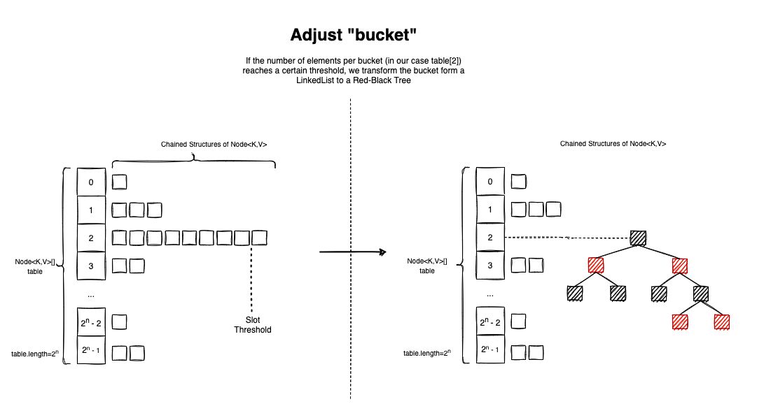
Another smart optimization the HashMap<K,V> performs is the Bucket Adjustment. The idea is simple - if the number of elements colliding inside a table slot (bucket) reaches a certain threshold, TREEIFY_THRESHOLD = 8, the pairs are re-organized in a red-black tree.

Searching in the tree is done in logarithmic time.

So let’s assume this optimization is ignored, and there are 64 elements in a bucket. Searching inside a linked list is O(n), so we will have to go through 64 iterations in the worst-case scenario. In a tree, searching is O(logn), so in the worst-case scenario, we will perform log₂2⁵= 5 operations.

Open Addressing

Compared to Separate Chaining, Open Addressing hash tables store only entry per slot. So there are no real buckets, no linked lists, and no red-black trees. It’s only one extensive array that has everything it needs to operate.

If the array of pairs is sparse enough (operating on a low load factor < 0.77), and the hashing function has decent diffusion, hash collisions should be rare. But even so, they can happen. In this case, we probe the array to find another empty slot for the entry to be inserted.

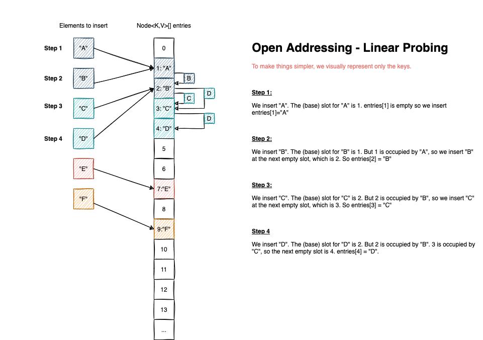
The most straightforward probing algorithm is called linear probing. In case of collision, we iterate over each bucket (starting with the first slot computed), until we find an empty index to make the insertion. If we reach the end of the array, we start again from index 0.

The advantage of Open Addressing over Separate Chaining is that cache misses are less frequent because we operate on a single contiguous block of memory (the array itself).

The visual representation for how inserts are working for Open Addressing is the following:

The biggest shortcoming for Open Addressing hash tables is that they are susceptible to lousy hash functions. Let think of it for a moment. The absolute worst hash function is one that returns a constant value. If it does so, all elements are going to target a single slot. We will have as many collisions as the number of elements.

In this case, the performance of HashMap<K,V> will have a graceful degrade to O(logn), while the performance of an Linear Probing hash table implementation will degrade to O(n).

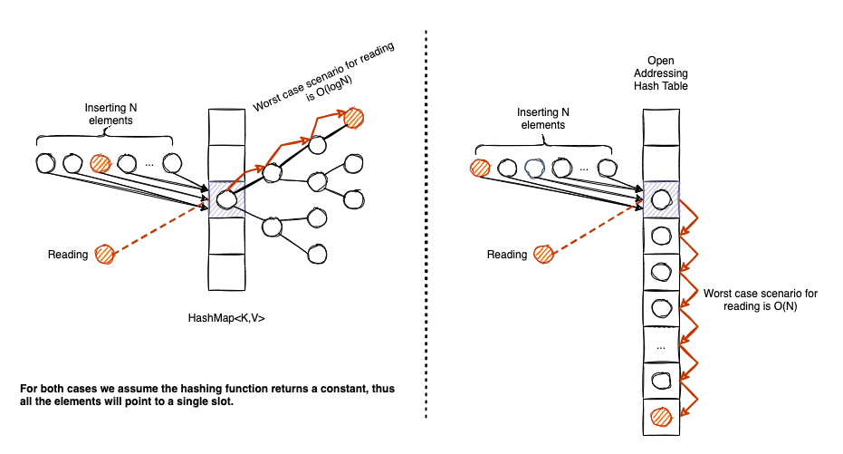
The above example is rather extreme, in practice, nobody will use a hash function that returns a constant integer. But if the hash function is sub-optimal, an Open Addressing (+Linear Probing) implementation is subject to what we call clustering: a dense area of occupied slots in our entries array that needs to be traversed in case of inserts/reads and deletes.

And one more thing before jumping straight to the code.

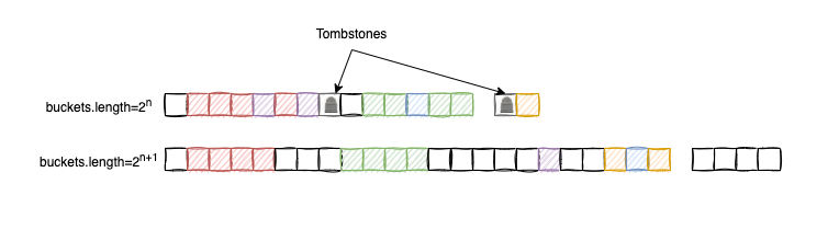
Deleting an element from an Open Addressing table is a subtle task! For this reason, we need to introduce the concept of tombstones (click on the link for an in-depth explanation).

Basically, whenever we delete an entry, we cannot empty the slot and make it null, because we might break an existing sequence. In this regard, we mark the slot as tombstone:

• If we are doing insert operations (put(Key k, V value)), we consider the tombstone a potential candidate for the insertion.
• If we perform read or delete operations, we skip the tombstone, and we continue the traversal to find the right spot.

Whenever we need to re-adjust the size of the entries array, we don’t rehash the tombstones. After all, they are “junk” elements introduced by delete operations.

Algorithms that avoid tombstones altogether exist, but they make the delete operation more complex, as they involve subsequent swaps of elements to fill up the space previously occupied by the deleted element. I’ve decided not to implement them. My logic was simple:

• In most of the cases, deleting an element from a Map<K,V> is not a common activity;
• If deletes are rare, introducing a few tombstones down the road won’t affect the performance in a significant manner.

LProbMap<K, V>

LProbMap<K,V> was my first academic attempt to implement an Open Addressing Map<K,V> in Java. I haven’t tried any trick; I’ve just implemented the corresponding algorithms by the book.

For the source code, check this link.

The first thing was to extend Map<K,V> and, as per the interface contract, I had to write an implementation for all the abstract methods. I won’t copy-paste the entire code here, but I will focus on the most important methods: put, get, remove, and the underlying data structures.

public class LProbMap<K, V> implements Map<K,V> {

    private static final double DEFAULT_MAX_LOAD_FACTOR = 0.6;
    private static final double DEFAULT_MIN_LOAD_FACTOR = DEFAULT_MAX_LOAD_FACTOR / 4;
    private static final int DEFAULT_MAP_CAPACITY_POW_2 = 6;

    private int size = 0;
    private int tombstones = 0;
    private int capPow2 = DEFAULT_MAP_CAPACITY_POW_2;

    public LProbMapEntry<K, V>[] buckets = 
                        new LProbMapEntry[1<< DEFAULT_MAP_CAPACITY_POW_2];

    // More code here
    
}

DEFAULT_MAX_LOAD_FACTOR is the maximum load factor my LProbMap<K,V> accepts. After this threshold is reached, the number of buckets is increased to the next power of two.

I’ve tried a few values, and 0.6 seems to be a decent choice for when I’ve benchmarked the read operations. At the same time, I am wasting 40% of my buckets array on null elements. 0.7 or 0.77 are also decent choices, so it’s up to you to try them out.

The loadFactor in for LProbMap<K,V> is computed by the following formula:

final double lf = (double)(size+tombstones) / buckets.length;

So compared to HashMap<K,V>, tombstones have an influence on this metric.

DEFAULT_MIN_LOAD_FACTOR is the minimum acceptable load factor before we reduce the size of buckets to the previous power of two.

DEFAULT_MAP_CAPACITY_POW_2 is the default power of two that we use to compute the capacity of the buckets (buckets.length == 1<<6 == 64).

An important aspect is to also define a static hash(Object object) function:

public static int hash(final Object obj) {
    int h = obj.hashCode();
    h ^= h >> 16;
    h *= 0x3243f6a9;
    h ^= h >> 16;
    return h & 0xfffffff;
}

As you can see, we (re)use Java’s obj.hashCode() method. We also apply a finalizer to it, inspired by Murmur Hash. The reason to shift/xor/multiply/shift/xor is to make better use of the high order bits of the object key.

The last line h & 0xfffffff ensures that the returned value is not a negative number. In Java, compared to C, for example, there is no uint32_t type, so we need to consider the sign. Doing this, we are invalidating (through others) the bit containing the sign.

In regards to the Map<K,V> contract, we need to use entries extending the Map.Entry<K,V> class.

protected static class LProbMapEntry<K, V> implements Map.Entry<K, V> {

    public K key;
    public V value;
    public int hash;

    public LProbMapEntry(K key, V value, int hash) {
        this.key = key;
        this.value = value;
        this.hash = hash;
    }

    // More code here
}

Inserting an entry

Inserting an entry in the LProbMap<K, V> is straightforward, and the algorithm is as follows:

• We increase capacity if the load factor is bigger than what we’ve decided to be the threshold;
• We compute the base bucket (slot);
  • If the bucket is null, we insert the element and increment the size;
  • Otherwise, we iterate forever (while(true)) using linear probing, until we either:
    • Find a tombstone to insert the entry, then we decrement the number of tombstones and increase the size. We return null;
    • Find an empty bucket, we increase the size. We return null;
    • Find the exact element, and we update the value. We return the oldVal.

The only difference to the HashMap<K,V> is that we don’t accept null keys. The reason is simple, we use entries with null keys as tombstones. This is our convention.

@Override
public V put(K key, V value) {
    if (null==key) {
        throw new IllegalArgumentException("Map doesn't support null keys");
    }
    return put(key, value, hash(key));
}

// This method is not called directly, so there's no need 
// to check if key is null
protected V put(K key, V value, int hash) {
    // We increase capacity if it's needed
    increaseCapacity();
    // We calculate the base bucket for the entry
    int idx = hash & (buckets.length-1);
    while(true) {
        // If the slot is empty, we insert the new item
        if (buckets[idx] == null) {
            // It's a free spot
            buckets[idx] = new LProbMapEntry<>(key, value, hash);
            size++;
            // No value was updated so we return null
            return null;
        }
        else if (buckets[idx].key == null) {
            // It's a tombstone
            // We update the entry with the new values
            buckets[idx].key = key;
            buckets[idx].value = value;
            buckets[idx].hash = hash;
            size++;
            tombstones--;
            // No value was updated so we return null
            return null;
        }
        else if (buckets[idx].hash == hash && key.equals(buckets[idx].key)) {
            // The element already existed in the map
            // We keep the old value to return it later
            // We update the element to new value
            V ret;
            ret = buckets[idx].value;
            buckets[idx].value = value;
            // We return the value that was replaced
            return ret;
        }
        // Linear probing algorithm
        // We jump to the next item
        // In case we've reached the end of the list 
        // we start again
        idx++;
        if (buckets.length==idx) idx = 0;
    }
}

In code above, one line that can look awkward, if you are not familiar with bitwise operations, is int idx = hash & (buckets.length-1). This is used to calculate the base slot for the entry. We define the base slot as the most natural position an entry could have in our buckets array, if there are no collisions.

LProbMap<K,V>.hash(Object key) will always return a positive integer in the interval [0, Integer.MAX_VALUE]. But we have only buckets.length slots available to insert the item. Typically, we could write hash(key) % buckets.length to return the base slot. But modulo % operation is kinda slow.

Multiplication and division take a longer time. Integer multiplication takes 11 clock cycles on Pentium 4 processors and 3 - 4 clock cycles on most other microprocessors. Integer division takes 40 - 80 clock cycles, depending on the microprocessor. Integer division is faster the smaller the integer size on AMD processors, but not on Intel processors. Details about instruction latencies are listed in manual 4: “Instruction tables”. Tips about how to speed up multiplications and divisions are given on pages 146 and 147, respectively. (source).

Honestly, I don’t know how the JVM is optimizing the code behind the scenes, so the best thing was to make sure optimizations were happening by using a simple bitwise trick.

Because buckets.length is a power of two, hash(key) % buckets.length is equivalent to writing hash(key) & (buckets.length -1). If you don’t believe me, just run the following code:

int size = 1 << 4; // 16
for(int i = 100; i < 1000; i++) {
    System.out.printf("%d %% %d = %d --- AND ---- %d & (%d -1) = %d\n", 
        i, size, i % size, i, size, i & (size-1));
}

// Output

// 100 % 16 = 4 --- AND ---- 100 & (16 -1) = 4
// 101 % 16 = 5 --- AND ---- 101 & (16 -1) = 5
// 102 % 16 = 6 --- AND ---- 102 & (16 -1) = 6
// 103 % 16 = 7 --- AND ---- 103 & (16 -1) = 7
// 104 % 16 = 8 --- AND ---- 104 & (16 -1) = 8
// 105 % 16 = 9 --- AND ---- 105 & (16 -1) = 9

// and so on

The trick has an easy visual explanation. Let’s look at an example, 1001 & (32-1) and why it’s equivalent with 1001 % 32:

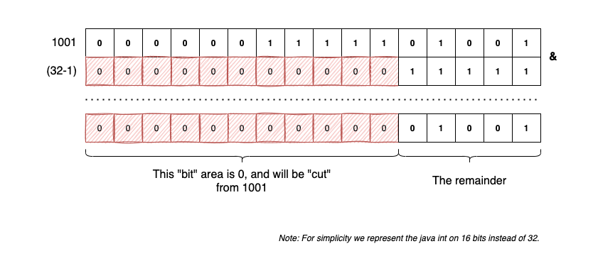
After the number is “cut”, the maximum value of 5 remaining bits is 31 (0...00011111).

Retrieving an entry

The algorithm for retrieving a V value by it’s Object key is the following:

• We compute the hash(key);
• We compute the base slot: idx = hash & (buckets.length-1);
• If the base slot is null, bucket[idx]==null , then we are 100% sure there’s no need to look further, and we return null;
• Otherwise, we check to see if the key’s hash matches the node’s hash
  • If they do, we do an additional check to see if the keys are equal. We do this extra step because there’s a small chance that two different elements have the same hash.
    • If not, we probe further;
    • If they are equals(), we return the V value;
• We repeat until we encounter a null slot, which means we’ve finished traversing the potential cluster of entries without finding what we were looking for.

public V get(Object key) {
    int hash = hash(key);
    // We determine the base bucket
    int idx = hash & (buckets.length-1);
    LProbMapEntry<K,V> bucket = buckets[idx];
    // If the base is null we return null
    if (bucket==null) {
        return null;
    }
    do {
        // If we found the element we return the value, 
        // breaking the loop
        if (bucket.hash == hash && key.equals(bucket.key)) {
            return bucket.value;
        }
        // We jump to the next element by using linear probing
        idx++;
        if (idx==buckets.length) idx = 0;
        bucket = buckets[idx];
    } while(null!=bucket);
    // We couldn't find any element,
    // We simply return null
    return null;
}

Deleting an entry

The algorithm for deleting an entry is as follows:

• We identify the base slot (the one bucket where we look first);
• If the base is null, there’s no reason to continue probing, we return null;
• Otherwise, we check to see if the slot’s hash matches the key’s hash. (If they do, we compare the keys using equals()).
  • If the element is present we remove it by inserting a tombstone;
  • We return the old value;
• We continue with the last step until the slot is null.
• We decrease the capacity if needed.

public V remove(Object key) {
     // We determine the base bucket
    int hash = hash(key);
    int idx = hash & (buckets.length-1);
    // If the base is null, there's no reason to continue probing
    // We simply return null
    if (null==buckets[idx]) {
        return null;
    }
    do {
        // If we found the bucket we insert a tombstone 
        // Increment the number of tombstones
        // and reduce the real size
        if (buckets[idx].hash == hash && key.equals(buckets[idx].key)) {
            V oldVal = buckets[idx].value;
            buckets[idx].key = null;
            buckets[idx].value = null;
            buckets[idx].hash = 0;
            tombstones++;
            size--;
            return oldVal;
        }
        // Continue with linear probing
        idx++;
        if (idx == buckets.length) idx = 0;
    } while (null != buckets[idx]);
    decreaseCapacity();
    return null;
}

Resizing and rehashing

We will follow the same trick as HashMap<K,V> in regards to capacity re-adjustment. If the load factor reaches a certain max threshold, we increase the capacity of the buckets to the next power of two. Vice-versa, if the load factor reaches a min threshold, we decrease the capacity of the buckets to the previous power of two. A full-rehashing is also happening.

Capacity re-adjustment is performed to reduce the clustering effect and to remove the previously inserted junk elements (tombstones). After a capacity re-adjustment, there are simply more slots available to insert the entries so the buckets array will become more sparse.

The code:

protected final void reHashElements(int capModifier) {
    // We modify the next power of two either +1 or -1
    this.capPow2+=capModifier;
    // We keep a reference to the old buckets
    LProbMapEntry<K, V>[] oldBuckets = this.buckets;
    // We allocate memory for new buckets
    this.buckets = new LProbMapEntry[1 << capPow2];
    this.size = 0;
    this.tombstones = 0;
    // We perform a full-rehash by re-insert all elements
    // We don't re-compute the hash, because it was already computed 
    for (int i = 0; i < oldBuckets.length; ++i) {
        if (null != oldBuckets[i] && oldBuckets[i].key != null) {
            this.put(oldBuckets[i].key, oldBuckets[i].value, oldBuckets[i].hash);
        }
    }
}

protected final void increaseCapacity() {
    final double lf = (double)(size+tombstones) / buckets.length;
    if (lf > DEFAULT_MAX_LOAD_FACTOR) {
        reHashElements(1);
    }
}

protected final void decreaseCapacity() {
    final double lf = (double)(size) / buckets.length;
    if (lf < DEFAULT_MIN_LOAD_FACTOR && this.capPow2 > DEFAULT_MAP_CAPACITY_POW_2) {
        reHashElements(-1);
    }
}

This approach is a little naive, but it works. It can be improved by computing in advance the actual value when we are going to trigger the rehash, so we don’t have to do final double lf = (double)(size) / buckets.length; at each insert/remove.

Also, depending on how many tombstones were created, we can reduce the capacity to reHashElements(-2) or reHashElements(-3) directly.

LProbSOAMap<K,V>

This is an interesting proposal made by dzaima on github.

For the full source code, please check the following link.

This is what we propose:

A very important property of open addressing is the ability to not need an allocation per inserted item. Without that, your LProbMap and Java’s HashMap differ only by where the next object pointer is read - a list in LProbMap, or the entry object in HashMap. Both are already in cache, so I would expect very similar performance, or worse because it has to iterate over more objects.

Here is a version of LProbMap utilizing a struct-of-arrays approach. It does mean that you have to read from three separate arrays, which would all be in different locations, but it’s the best Java can currently offer.

So we keep everything identical with LProbMap<K,V>, except we organize the memory in a different way.

Instead of defining a single LProbMapEntry<K, V>[] buckets array of buckets, we split the data into three arrays:

public K[] bucketsK = (K[]) new Object[1<<DEFAULT_MAP_CAPACITY_POW_2];
public V[] bucketsV = (V[]) new Object[1<<DEFAULT_MAP_CAPACITY_POW_2];
public int[] bucketsH = new int[1<<DEFAULT_MAP_CAPACITY_POW_2]; // k=null: hash=0 - empty; hash=1 - tombstone

In this way, we are not forced to use Map.Entry<K,V> and opt for a more straightforward memory layout.

PerturbMap<K, V>

PerturbMap<K,V> is my second approach of implementing an Open Addressing Map<K,V>, and it’s almost identical to LProbMap<K,V> with one significant change.

Reading the source code for cpython’s dict implementation I’ve stumbled upon those lines:

(...)

This is done by initializing a (unsigned) vrbl "perturb" to the

full hash code, and changing the recurrence to:

    perturb >>= PERTURB_SHIFT;
    j = (5*j) + 1 + perturb;
    use j % 2**i as the next table index;

(...)

To avoid clustering (that depends on how good our hash function is), a new strategy for probing is proposed, one that doesn’t use linear probing, but instead tries to scramble the entries positions by itself.

So instead of cycling through the array with:

idx++
if (idx == buckets.length) idx = 0;

We will do something like:

idx = 5 * idx + 1 + perturb;
perturb>>= SHIFTER;
idx = idx & (buckets.length-1);

Where SHIFTER is a constant, that equals to 5, and peturb is initialized to peturb=hash.

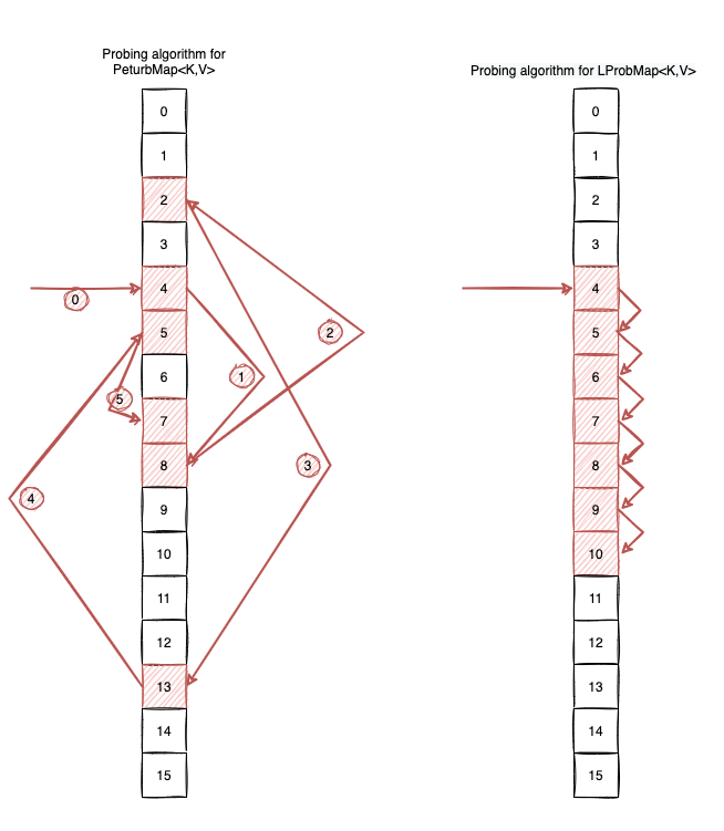
To make things clearer, let’s look at the following example. Let’s assume our initial hash=32132932, shifter=5 and bucketsLength=1<<4. Let’s see how the probing goes if we use this algorithm:

final int hash = 32132932;
final int shifter = 5;
final int bucketsLength = 1 << 4;

int idx = hash & (bucketsLength-1);
System.out.println(idx);

int j = 5;
int perturb = hash;
while(j-->0) {
    idx = 5 * idx + perturb;
    perturb>>=shifter;
    idx = idx & (bucketsLength-1);
    System.out.println(idx);
}

The output is:

4 8 2 13 5 7

Visually, the probing algorithm looks like this:

You can access all the code here, but as an example, this is how the get(Object key) looks like:

public V get(Object key) {
    if (null==key) {
        throw new IllegalArgumentException("Map doesn't support null keys");
    }
    int hash = hash32(key);
    int idx = hash & (buckets.length-1);
    if (null == buckets[idx]) {
        return null;
    }
    int perturb = hash;
    do {
        if (buckets[idx].hash == hash && key.equals(buckets[idx].key)) {
            return buckets[idx].value;
        }
        // !! Different than LProbMap<K,V> !!
        idx = 5 * idx + 1 + perturb;
        perturb>>= SHIFTER;
        idx = idx & (buckets.length-1);
    } while (null != buckets[idx]);
    return null;
}

Now, in terms of performance:

• We combat clustering by augmenting the diffusion of the hashing function with this simple trick;
• We potentially increase the number of cache misses, because elements that were previously sharing the same locality are now spread across the buckets.

LProbBinsMap<K,V>

This is another almost identical implementation to LProbMap<K,V>, but with an extra change inspired by ruby’s hash table implementation. For simplicity, I’ve opted to use linear probing as the probing algorithm.

For the full source code please check this link

The main idea is to avoid keeping everything inside the buckets array, so we split the information between two arrays:

• int[] bins
• Map.Entry<K,V>[] entries

bin is (sparse) array of integer values that where we keep the indices of the entries.

entries is an ArrayList<Map.Entry<K,V>>-like structure, that is dense. Here is were we store the actual keys, values, hashes.

Visually LProbBinsMAp<K,V> looks like this:

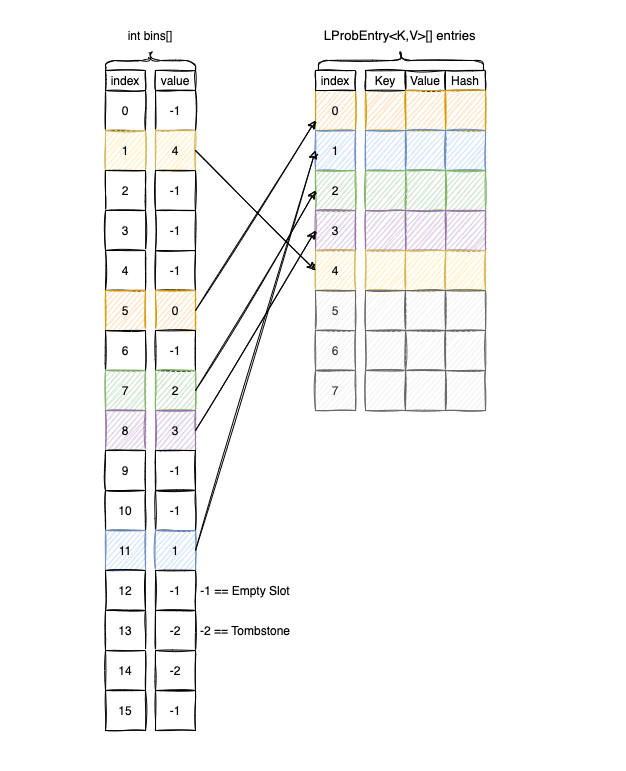
To find the base bucket we do a look-up inside bins, where we keep the index of entries.

Code wise, this is only a re-interpretation of LProbMap<K,V. As an example this is how the get(Object key) method looks like:

public V get(Object key) {
    if (null==key) {
        throw new IllegalArgumentException("Map doesn't support null keys");
    }
    int hash = hash(key);
    int idx = hash & (bins.length-1);
    if (bins[idx]==EMPTY_SLOT) {
        return null;
    }
    do {
        if (bins[idx]!=TOMBSTONE && entries[bins[idx]].hash==hash && key.equals(entries[bins[idx]].key)) {
            return entries[bins[idx]].value;
        }
        idx++;
        if (idx == bins.length) idx = 0;
    } while(bins[idx]!=EMPTY_SLOT);
    return null;
}

The advantage of this approach should be reduced memory consumption and increased memory locality.

LProbRadarMap<K, V>

LProbRadarMap<K,V> is an original attempt to write an implementation for Map<K,V>, that fights clustering, by keeping a radar like structure that tracks the neighborhood of an element.

For the full source code please check this link

The radar[i] keeps track of all the elements of buckets that have the base in i and are spread in the next 32 positions.

To better understand, let’s look at the following diagram:

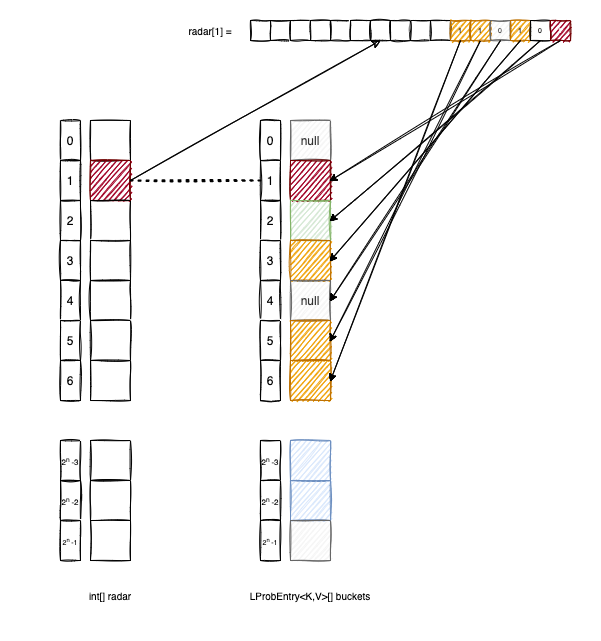
buckets[2] doesn’t have the base in 1, so the second bit of radar[1] is 0.

bucket[3], buckets[5] and buckets[6] have the base in 1, so we set to 1 the corresponding bits in radar[1].

Inserting an element in the LProbRadarMap<K,V> looks like this:

protected V put(K key, V value, int hash) {
    // We increase the capacity if needed
    if (shouldGrow()) {
        grow();
    }
    int idx = hash & (buckets.length-1);
    int base = idx;
    int probing = 0;
    while(true) {
        // We increase the capacity if we exit the radar
        if (probing==32) {
            grow();
            return put(key, value, hash);
        }
        if (buckets[idx] == null) {
            // It's a free spot
            buckets[idx] = new LProbEntry(key, value, hash);
            // We mark the bit in the radar entry
            radar[base] |= (1 << probing);
            size++;
            return null;
        }
        else if (buckets[idx].key == null) {
            // It's a tombstone
            buckets[idx].key = key;
            buckets[idx].val = value;
            buckets[idx].hash = hash;
            radar[base] |= (1 << probing);
            size++;
            tombstones--;
        }
        else if (buckets[idx].hash == hash && key.equals(buckets[idx].key)) {
            // We perform an update on the element
            V ret;
            ret = buckets[idx].val;
            buckets[idx].key = key;
            buckets[idx].hash = hash;
            buckets[idx].val = value;
            return ret;
        }
        probing++;
        idx++;
        if (buckets.length==idx) idx = 0;
    }
}

The algorithm for retrieving an element from LProbRadarMap<K,V> is the following:

public V get(Object key) {
    if (null==key) {
        throw new IllegalArgumentException("Map doesn't support null keys");
    }
    int hash = hash(key);
    int idx = hash & (buckets.length-1);
    int rd = radar[idx];
    if (rd==0) {
        return null;
    }
    for(int bit = 0; bit < 32; bit++) {
        if (((rd>>bit)&1)==1 && buckets[idx].hash == hash && key.equals(buckets[idx].key)) {
            return buckets[idx].val;
        }
        idx++;
        if (idx == buckets.length) idx = 0;
    }
    return null;
}

To be honest, doing this doesn’t achieve much because doing the bit check (rd>>bit)&1)==1 is not necessarily more efficient than just verifying if the bucket[idx]is null.

Also, enforcing this:

if (probing==32) {
    grow();
    return put(key, value, hash);
}

it’s dangerous approach. We have no control on how the inserted Object key implements its hashCode(), so a bad hashCode() function might form clusters bigger than 32 (which is the maximum radar size for each element). In this regard, our buckets array can grow indefinitely until eventually crashing with an OOM.

Nevertheless, it was a fun exercise.

RobinHoodMap<K, V>

This was my last attempt at implementing an Open Addressing hash table, using the Robin Hood hashing technique.

For the full source code please check this link

Robin Hood works exactly as Linear Probing, with one more addition. When we insert a new entry, we also keep track of how it is from its base. In this regard, we add a new attribute to the inner Map.Entry<K,V>:

public static class Entry<K, V> implements Map.Entry<K, V> {

    private K key;
    private V value;
    private int hash;
    private int dist; // <--

    // (more code)
}

dist signifies the distance of the entry from its base.

Whenever a new entry is inserted, we try to put it as close as possible to its base slot, displacing older entries in the process and putting them closer to the clusters’ edge.

Let’s look at the following example:

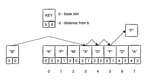
• We want to insert "B". The base slot for "B" is 3.
• We try to insert "B" at index 3. But distance(B,3) == 0 < distance(X,2) == 1 so we don’t do a swap;
• We try to insert "B" at index 4. But distance(B,3) == 1 < distance(D,2) == 2 so we don’t do a swap;
• We try to insert "B" at index 5. distance(B,3) == 2 > distance(F,4) == 1 so we swap B with F and we continue in the same manner to insert F.

The get and remove operations are exactly as for LProbMap<K,V>, but what it differs is the put operation:

protected V put(K key, V value, int hash) {
    if (null==key) {
        throw new IllegalArgumentException("Map doesn't support null keys");
    }
    increaseCapacity();
    K cKey = key;
    V cVal = value;
    int cHash = hash;
    V old = null;
    int probing = 0;
    // Identifying the base slot
    int idx = hash & (buckets.length - 1);
    while (true){
        // If the bucket is empty we simply insert the element and we break the loop
        if (null == buckets[idx]) {
            buckets[idx] = new Entry<>(cKey, cVal, cHash, probing);
            this.size++;
            break;
        } 
        // If we found the bucket, we just update the value
        else if (hash == buckets[idx].hash && key.equals(buckets[idx].key)) {
            old = buckets[idx].value;
            buckets[idx].value = value;
            buckets[idx].dist = probing;
            break;
        } 
        // We probe & swap until we find the right slot
        else if (probing > buckets[idx].dist) {
            K tmpKey;
            V tmpVal;
            int tmpHash;
            int tmpDist;
            tmpHash = buckets[idx].hash;
            tmpVal = buckets[idx].value;
            tmpDist = buckets[idx].dist;
            tmpKey = buckets[idx].key;
            buckets[idx].hash = cHash;
            buckets[idx].value = cVal;
            buckets[idx].key = cKey;
            buckets[idx].dist = probing;
            cHash = tmpHash;
            cVal = tmpVal;
            cKey = tmpKey;
            probing = tmpDist;
        }
        // Linear probing is used
        probing++;
        idx++;
        if (idx == buckets.length) idx = 0;
    }
    return old;
}

One significant advantage of Robin Hood hashing is that it enforces minimal variances of entries compared to their base slot. There are no worst-case scenarios whenever we get an element because all elements will have almost the same distance for a given base slot.

Benchmarks

After having implemented the five six Open Addressing maps, (LProbMap.java, LProbBinsMap.java, LProbRadarMap.java, PerturbMap.java, RobinHoodMap.java), I wanted to check how good they perform vs. the HashMap<K,V> reference implementation.

(micro)Benchmarking in Java is hard, so in this regard, I’ve used jmh + mockneat (to generate test data).

The benchmarks are included in the repo, so if you plan to check out the code:

git clone git@github.com:nomemory/open-addressing-java-maps.git

they can be found in the performance/jmh folder.

If you want to run them yourself, see the Main.class.

// Cleans the existing generated data from previous runs
InputDataUtils.cleanBenchDataFolder();

Options options = new OptionsBuilder()
        // Benchmarks to include
        .include(RandomStringsReads.class.getName())
        .include(SequencedStringReads.class.getName())
        .include(AlphaNumericCodesReads.class.getName())
        // Configuration
        .timeUnit(TimeUnit.MICROSECONDS)
        .shouldDoGC(true)
        .resultFormat(ResultFormatType.JSON)
        .addProfiler(GCProfiler.class)
        .result("benchmarks_" + System.currentTimeMillis() + ".json")
        .build();

new Runner(options).run();

At the end of the program execution, a benchmark_*.json file will be generated (but be prepared; it will take some time).

You can visually analyze the results by using this tool or running this quick python script.

At the moment I am writing this article, there are three benchmark classes:

• RandomStringsReads
• SequencedStringReads
• AlphaNumericCodesReads

They are configured like this:

@BenchmarkMode(Mode.AverageTime)
@OutputTimeUnit(TimeUnit.MICROSECONDS)
@State(Scope.Benchmark)
@Fork(value = 3, jvmArgs = {"-Xms6G", "-Xmx16G"})
@Warmup(iterations = 2, time = 5)
@Measurement(iterations = 4, time = 5)

We use 3 forks, 2 warmup iterations, and 4 measurements. I know I should’ve probably increased those values, but even like this, and given the high input params variance, the benchmark takes around 6 hours to complete on my machine.

To conclude, I believe this is enough to get a glimpse of the performance of the code.

Each benchmark class has two methods:

@Benchmark
@CompilerControl(CompilerControl.Mode.INLINE)
public void randomReads(Blackhole bh) {
    bh.consume(
            testedMap.get(fromStrings(keys).get())
    );
}

@Benchmark
@CompilerControl(CompilerControl.Mode.INLINE)
public void randomReadsWithMisses(Blackhole bh) {
    bh.consume(
            testedMap.get(fromStrings(keysWithMisses).get())
    );
}

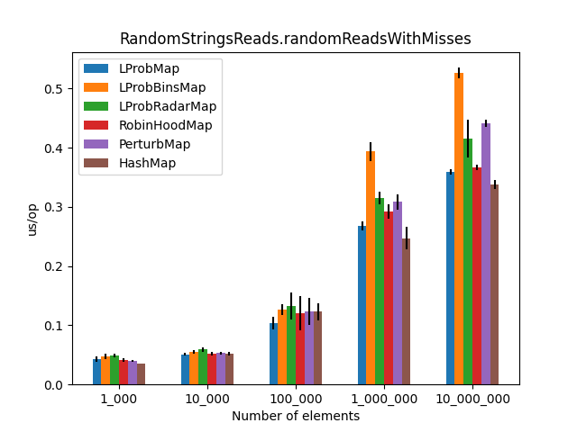
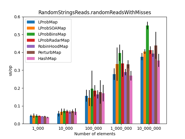
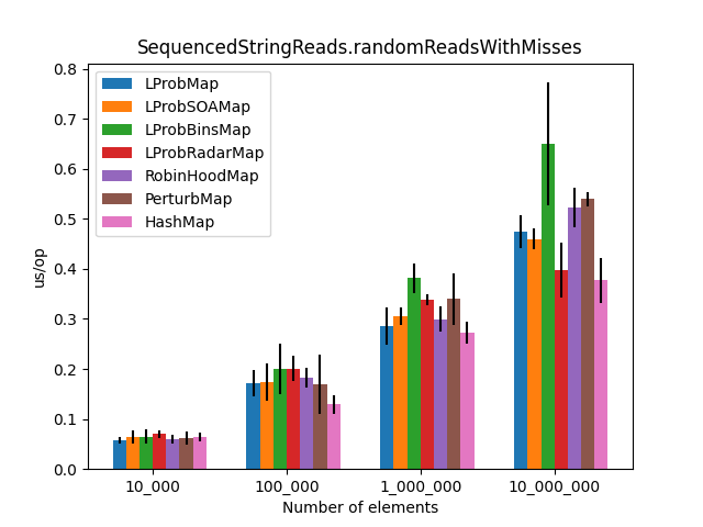
The randomReadsWithMisses() method benchmarks get() operations where keys have a 50% chance of not being present in the Map<K,V>.

For randomReads(), it is guaranteed all the keys exist.

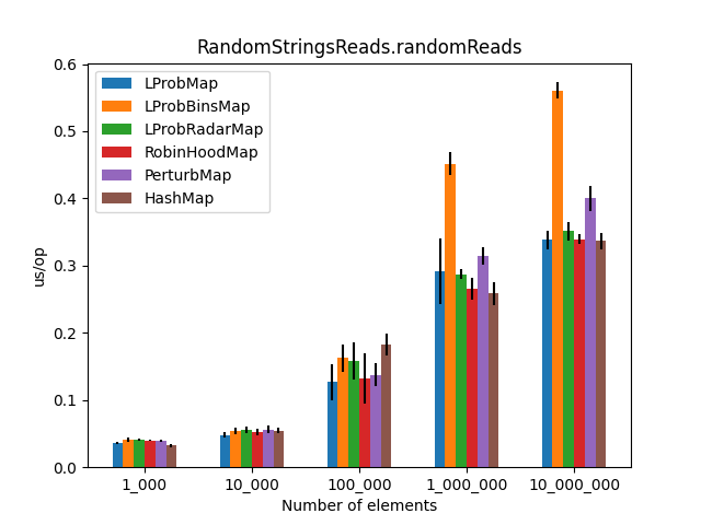
RandomStringsReads

The full code of this benchmark can be found here.

For this benchmark the keys are randomly generated by following this simple rule:

 probabilities(String.class)
            .add(0.2, names().full())
            .add(0.2, addresses())
            .add(0.2, words())
            .add(0.2, cars())
            .add(0.2, ints().mapToString())

probabilities() is a mockneat method that generates random data based on given “chances”.

The keys are String values that:

• Have a 20% chance of being full names (e.g., “Mike Smith”);
• Have a 20% chance of being a full address;
• Have a 20% chance of being a random word from the English dictionary;
• Have a 20% chance of being a “car” name and model;
• Have a 20% chance of being a numerical value (an int) converted to String.

This benchmark will have the following input params:

@Param({"KEYS_STRING_1_000", "KEYS_STRING_10_000", "KEYS_STRING_100_000", "KEYS_STRING_1_000_000", "KEYS_STRING_10_000_000"})
private StringsSourceTypes input;

@Param({"LProbMap", "LProbBinsMap", "LProbRadarMap", "RobinHoodMap", "PerturbMap", "HashMap"})
private MapTypes mapClass;

KEYS_STRING_1_000 means that data will be read from a MapType={LProbMap, LProbBinsMap, ...} with 1000 entries, KEYS_STRING_10_000 means that data will be read from a MapType={LProbMap, LProbBinsMap, ...} with 10_000 entries, and so on, up to 10_000_000 entries.

Note: I’ve created the benchmarks in such a way, the same data will be used for all the MapTypes.

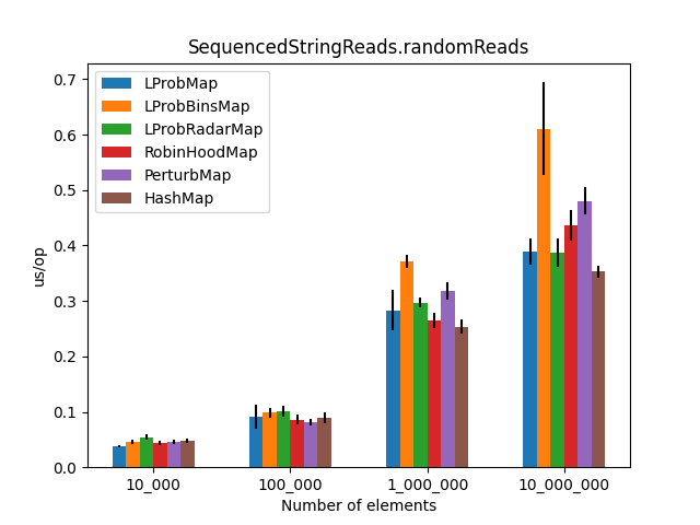
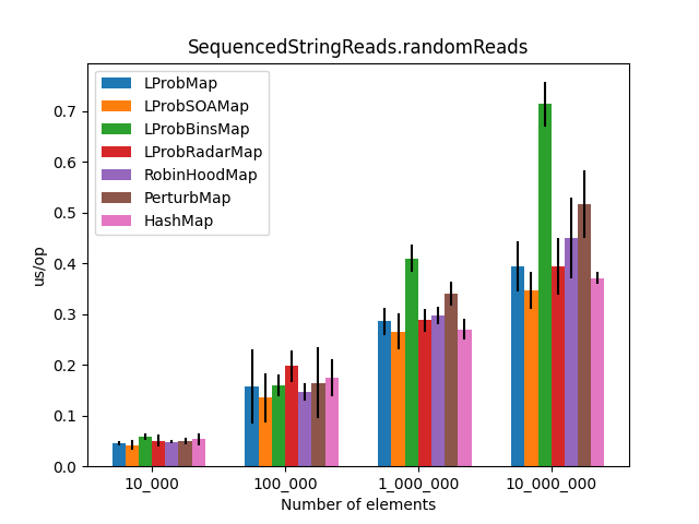
SequencedStringsReads

The full code of this benchmark can be found here.

For this benchmark, the keys are randomly generated by following this simple rule:

intSeq().mapToString()

intSeq() is part of the mockneat API.

Basically the keys will be String values that are int values in a sequence: "0", "1", …, "1000".

The reason I’ve introduced this benchmark was to see how my Maps are performing versus input that has a certain pattern.

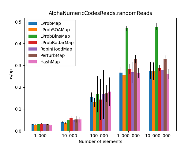
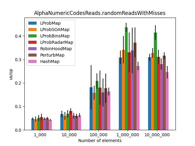
AlphaNumericCodesReads

The full code of this benchmark can be found here.

For this benchmark, the keys are randomly generated by following this simple rule:

strings().size(6).type(StringType.ALPHA_NUMERIC)

Keys are alphanumeric characters of length==6.

I’ve introduced this benchmark (again) to see how my Maps are performing versus input with specific patterns.

The results

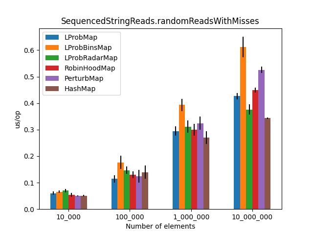
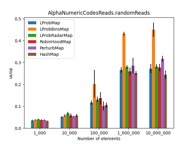
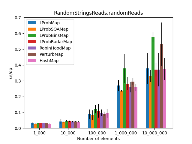
After running all the three benchmarks for almost 6 hours, I’ve got the following results:

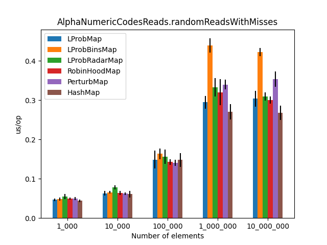The results (2)

After the LProbMapSOA<K,V> contribution from dzaima, I’ve decided to re-run the benchmarks and include it. The new results are:

Wrapping up

Firstly, the benchmarks are incomplete as we haven’t tested the performance for put or remove operations. More work can be done to improve both methods. The tombstones strategy is probably not the best; more thoughtful implementations prefer shifting elements instead.

Secondly, I was surprised to see that LProbMap<K,V> and RobinHoodMap<K,V> are performing relatively well vs. HashMap<K,V> for datasets < 1_000_000. After the number of elements increases, performance is degrading but not by huge margins. In terms of memory consumption, the results were also quite similar.

Implementing the five six Open Addressing maps was a fun and frustrating exercise. In Java, you can only be half-smart when you are writing code. The other half is where the JIT comes into play. You cannot control even what function is getting inlined. So writing the code to make it as fast as possible was a trial and error endeavor. I am not even sure I’ve made the right decisions.

I had high hopes for LProbBinsMap<K,V>, but surprisingly it performed the worst. Maybe I’ve missed something and someone more experienced than me can find the reason why it works poorly.

LProbSOAMap<K,V> performed exceptionally well, especially when we query entries that exist on the Map<K,V>. It performed better than LProbMap<K,V> and even HashMap<K,V> when the number of elements is lesser than 10_000_000. Afterward, HashMap<K,V> starts to shine.

Should you ever consider using an Open Addressing hash table in Java instead of HashMap<K,V>. Probably not. HashMap<K,V> is simple, performant and bullet-proof.

I am yet to find an Open Addressing implementation that outperforms HashMap<K,V> by a significant margin. If you have additional ideas, you can use the existing repo, as you already have some infrastructure at hand: unit tests, benchmarks, and a script to plot the results. I am accepting PRs, and I will update the article.

Discussion

Related hacker news link.

Related reddit link.