Linear transformations, Eigenvectors and Eigenvalues - an easy explanation

This article is in early editing. It may suffer changes or corrections. If you spot any error please contact me.

There are rumors saying Computer Vision Engineers consider Eigenvalues and Eigenvectors the single most important concept(s) in linear algebra. I am not 100% sure about that, but I must admit those two things confused me a lot during my university years.

I think my teacher lost me somewhere in between The basis of a vector space and Linear transformations. N-dimensional vectors rotating ?! That was too much for me. So I’ve stopped caring, learned the formulas, and passed the exam. So here I am more than ten years later, interested in A.I. algorithms and realizing those two notions are much simpler than I’ve thought.

But, before jumping directly into the subject, we must first talk about a few auxiliary concepts that will help us better understand the mystery behind Eigenvectors and Eigenvalues.

Think of matrices as functions f(x) = …

In mathematics, a function is a rule that accepts an input and produces an output.

For example \(f(x) = x + 1 , f : N \rightarrow N\) is a function that accepts a natural number x, increments the number with 1 and returns the result. As expected \(f(0) = 0 + 1 = 1\) and \(f(5) = 5 + 1 = 6\). If x varies, then the result will vary.

Now let’s think of matrix A with m rows and n columns (A[mxn]), and we consider the following equation \(b=A * x\) where:

• x is an n-dimensional vector, \(x \in R^n\)
• b is an m-dimensional vector, \(b \in R^m\)

Looking closer, we can see that if we change x, b will probably be changed. So A acts exactly like a function.

Forcing the mathematical notation a little, we can say \(A(x) = b \text{,where } A : R^n \rightarrow R^m\).

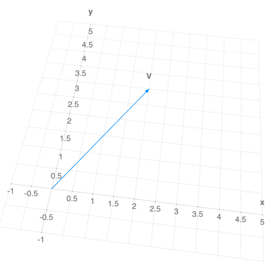
Example 1:

Let’s consider a bi-dimensional vector \(V = \begin{bmatrix} 2 \\ 3 \end{bmatrix} \text{, where } V \in R^2\).

If we were to plot this vector in the 2-d plane, it would look like this:

Now, let’s define a matrix A = \(\begin{bmatrix} 1 & 0 \\ 0 & 0 \end{bmatrix}\) and we compute \(A * V\):

\(V^{'}= \begin{bmatrix} 1 & 0 \\ 0 & 0 \end{bmatrix} * \begin{bmatrix} 2 \\ 3 \end{bmatrix} = \begin{bmatrix} 2 \\ 0 \end{bmatrix} \text{ ,where } V^{'} \in R^2\).

As we can see, applying the “matrix” function to our vector, \(A(V)=V^{'}\), we removed the y information from it. So if we plot it in the two-dimensional space:

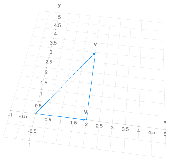
We can observe that \(V^{'}\) is the \(V\) projection on the x-axis of our system, thus the matrix A works as a function that projects any vector to the x-axis.

A works the same for every vector \(V = \begin{bmatrix} x \\ y \end{bmatrix} \text{ ,where } V \in R^2\), it will always retrieve the orthogonal projection of point (x, y) on the x-axis.

Matrix transformations

A transformation \(T\), is a “rule” that assigns to each vector \(v \in R^n\) a vector \(T(v) \in R^m\).

• \(T(x) \in R^m\) is the image of \(x \in R^n\) under \(T\);
• All images \(T(x)\) are called the range of \(T\);
• \(R^n\) is the domain of \(T\);
• \(R^m\) is the co-domain of \(T\);

n is not necessarily different than m, as we saw in our previous example.

Let A be an nxm matrix. The matrix transformation associated with A is the transformation: \(T : R^n \rightarrow R^m \text{ ,defined by } T(x) = A * x\).

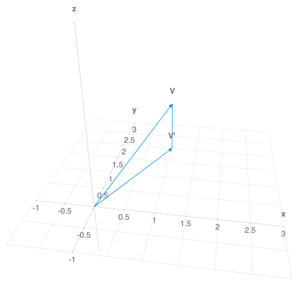
Example: Projection on the (x, y) plane

Let A[3x3] be:

\[A= \begin{bmatrix} 1 & 0 & 0 \\ 0 & 1 & 0 \\ 0 & 0 & 0 \\ \end{bmatrix}\]

If we form the matrix transformation equation \(A * v = b \text{ ,where } v \in R^3\):

\[A * v = \begin{bmatrix} 1 & 0 & 0 \\ 0 & 1 & 0 \\ 0 & 0 & 0 \end{bmatrix} * \begin{bmatrix} x \\ y \\ z \end{bmatrix} = \begin{bmatrix} x \\ y \\ 0 \end{bmatrix} = v^{'}\]

We see that the z information of our vector \(v\) has “evaporated”. The matrix \(A\) projected our vector \(v\) on the <x, y> plane.

To visualise better, let’s say \(v=\begin{bmatrix}1 \\ 2 \\ 1\end{bmatrix}\) and we plot \(v^{'} = A * v = \begin{bmatrix}1 \\ 2 \\ 0\end{bmatrix}\):

Linear Transformations

A linear transformation is a Transformation \(T:R^n \rightarrow R^m\) satisfying the following conditions:

\[T(u+v) = T(u) + T(v) \\ T(cu) = c * T(u)\]

where \(u, v \in R^n\) and \(c\) is a scalar.

If we write this with a matrix notation, given \(T(x) = A*x =>\), we have:

\[A(u+v) = A * u + A * v \\ A(c*u) = c * A * u\]

• It’s important to remember that a linear transformation takes the zero vector to the zero vector: \(T(0) = 0\)
• Also, for all/any vectors \(v_{1}, v_{2}, ..., v_{n}\) from \(R^n\), and scalars \(c_{1}, c_2{}, ..., c_{n}\) we have: \(T(c_{1}*v_{1} + c_{2}*v_{2}+ ... + c_{k}*v_{k}) = c_{1} * T(v_{1}) + c_{2} * T(v_{2}) + ... + c_{k} * T(v_{k})\).

At this point, it’s important to note that not all the transformations we’ve discussed are linear transformations.

For example a “translation” in the form: \(T(x) = x + \begin{bmatrix} 1 \\ 2 \\ 3 \end{bmatrix}\) is not a linear transformation, because \(T(0) = \begin{bmatrix} 1 \\ 2 \\ 3 \end{bmatrix} => T(0) != 0\).

But without going into all the demonstration, we can state something very important:

Every linear transformation is a matrix transformation!

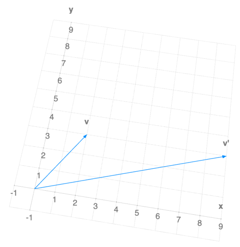
For example the matrix \(A = \begin{bmatrix} 3 & 1 \\ 1 & 2 \end{bmatrix}\) describes a linear transformation because:

\[A * [0] = [0] \text{, and}\\ A(u + v) = \begin{bmatrix} 3 & 1 \\ 1 & 2 \end{bmatrix} * \begin{bmatrix} u_{1} + v_{1} \\ u_{2} + v_{2} \end{bmatrix} = \begin{bmatrix} 3 * (u_{1} + v_{1}) + (u_{2} + v_{2}) \\ (u_{2} + v_{2}) + 2 * (u_{2} + v_{2}) \end{bmatrix} =\\ \begin{bmatrix} (3 * u_{1} + u_2{}) + (3 * v_{1} + v_{2}) \\ (u_{1} + 2 * u_{2}) + (v_{1} + 2 * v_{2}) \end{bmatrix} =\\ A * v + A * u\]

If we apply this linear transformation to an existing vector \(v=\begin{bmatrix} 1 \\ 2\end{bmatrix}\) the resulting vector will be:

\[v^{'}= \begin{bmatrix} 3 & 1 \\ 1 & 2 \end{bmatrix} * \begin{bmatrix} 1 \\ 2 \end{bmatrix} = \begin{bmatrix} 5 \\ 5 \end{bmatrix}\]

To visualise \(v\) and \(v^{-1}\) we can plot them together:

As you can see the initial vector was “stretched”, and changed it’s span.

Eigenvalues and Eigenvectors

Let there be a transformation matrix A[nxn]. We say:

• An eigenvector is a non zero vector \(v \in R^n\), and the equation \(A * v = \lambda * v\) is true, for some scalar \(\lambda\).
• An eigenvalue of \(A\) is a scalar \(\lambda\), so that the previous equation \(A * v = \lambda * v\) has a non-trivial solution.

Looking at the equation \(A * v = \lambda *v\) we can say that an eigenvector of linear transformation is a “characteristic vector” (something intrinsically related with the transformation) that changes by a scalar factor when that linear transformation is applied to it. The corresponding scalar, \(\lambda\), that stretches the vector is the eigenvalue.

The process of computing the eigenvectors and eigenvalues can be the following

\[A * v = \lambda * v\\ A * v = (\lambda * I) * v \\ A * v - (\lambda * I) * v = 0 \\ (A - \lambda * I) * v = 0 \\ \text{determinant(} A - \lambda * I\text{)} = 0\]

Let’s take the matrix \(A = \begin{bmatrix} 3 & 1 \\ 0 & 1 \end{bmatrix}\) as an example.

After calculating \(A - \lambda * I = \begin{bmatrix} 3 - \lambda & 1 \\ 0 & 1 - \lambda \end{bmatrix}\), we need to check the solutions of \(\lambda\) for which the \(det(A - \lambda * I) = 0\).

But \(det(A - \lambda * I) = (3 - \lambda) * (1 - \lambda) = 0\), thus we find the two eigenvalues \(\lambda_{1}=3, \lambda_{2}=1\).

Now that we have the eigenvalues, we can compute the two eigenvectors, but solving two linear systems of equations in the form:

\[\begin{bmatrix} 3 - 1 & 1 \\ 0 & 1 - 1 \end{bmatrix} * \begin{bmatrix} v_{1x} \\ v_{1y} \end{bmatrix} = \begin{bmatrix} 0 \\ 0 \end{bmatrix} \\ \begin{bmatrix} 3 - 3 & 1 \\ 0 & 1 - 3 \end{bmatrix} * \begin{bmatrix} v_{2x} \\ v_{2y} \end{bmatrix} = \begin{bmatrix} 0 \\ 0 \end{bmatrix}\]

If we solve the two systems of equations, we will realize that our matrix “A” has multiple eigenvectors/eigenvalues pairs.

\[\text{For } \lambda_{1} = 1 \text{, we have the eigenvectors } v_{1} = \begin{bmatrix} x \\ -2x \end{bmatrix} = \begin{bmatrix} \frac{-1}{2} \\ 1 \end{bmatrix} * x\\ \text{For } \lambda_{2} = 3 \text{, we have the eigenvectors } v_{2} = \begin{bmatrix} x \\ 0 \end{bmatrix} = \begin{bmatrix} 1 \\ 0 \end{bmatrix} * x\]

Wait! If you look closer, the eigenvalues \(\lambda_{1}=1\) and \(\lambda_{2}=3\) are exactly the elements of the first diagonal of our matrix \(A\). That’s not a pure coincidence. The matrix \(A\) is an upper diagonal matrix (has only zero elements under the first diagonal). So we can generalize the following: the eigenvalues for a diagonal matrix are the elements of the first diagonal.

Now, we can visually see why eigenvectors are so “special”.

Using our transformation \(A= \begin{bmatrix} 3 & 1 \\ 0 & 1 \end{bmatrix}\) on a “normal”, “non-eigenvector” vector \(v = \begin{bmatrix} 2 \\ 3 \end{bmatrix}\), we obtain a new vector \(v' = \begin{bmatrix} 3 & 1 \\ 0 & 1 \end{bmatrix} * \begin{bmatrix} 2 \\ 3 \end{bmatrix} = \begin{bmatrix} 9 \\ 3 \end{bmatrix}\), and project:

We see that \(v_{1}\) changed its span in comparison with the initial \(v\), from before the transformation.

But on the contrary if we use a eigenvector \(v_{eig} = \begin{bmatrix} 2 \\ 0 \end{bmatrix} = v_{eig}^{'}\), and we apply the transformation associated with \(A\) on it: \(A * v_{eig} = \begin{bmatrix} 3 & 1 \\ 0 & 1 \end{bmatrix} * \begin{bmatrix} 2 \\ 0 \end{bmatrix} = \begin{bmatrix} 6 \\ 0 \end{bmatrix}\), and we project:

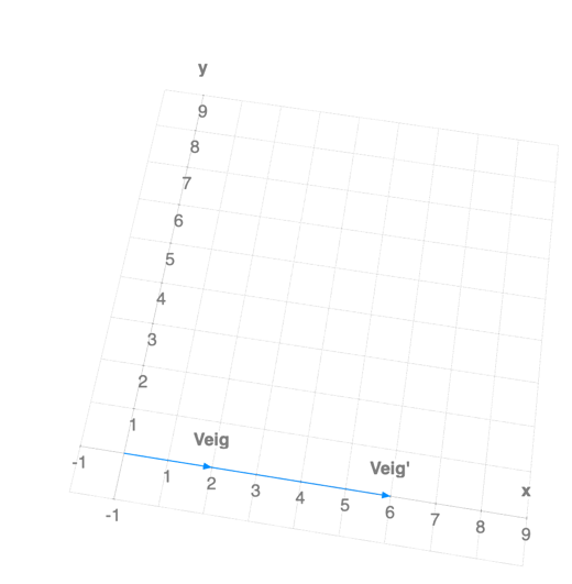
We can see that \(v_{eig}^{'}\) didn’t change its span compared to \(v_{eig}\).

Conclusion: Eigenvectors and Eigenvalues are essential because, in a way, they act like an “axis”, along which a linear transformation works simply by “shrinking/stretching” and not performing any other alterations.

So Eigenvectors helps us model and understand the complex ways in which a linear transformation work by decoupling their actions into “independent” “axes”.

Not every linear transformation has “real” eigenvectors, but all linear transformations have “complex” eigenvectors.

For example the matrix associated with a linear transformation that performs a planar rotation clockwise is \(A = \begin{bmatrix} 0 & 1 \\ -1 & 0 \end{bmatrix}\).

If we compute the eigenvalues for \(A\) we will obtain: \(\lambda_{1}=-i\) and \(\lambda_{2}=i\). In this case the two associated eigenvectors will be: \(v_{1} = \begin{bmatrix} i \\ 1 \end{bmatrix}\) and \(v_{2} = \begin{bmatrix} -i \\ 1 \end{bmatrix}\).

The results are not surprising because \(A\) will rotate every vector, and the span of the vector changes automatically.

Why are Eigenvectors and Eigenvalues important

From a “Computer Engineering” perspective, Eigenvectors and Eigenvalues are important in the following areas:

• Statistics;
• Computer Vision (e.g., Principal Component Analysis);
• Image compression.
• etc.

Where to go next

If you want to find out how to compute Eigenvectors and Eigenvalues, please refer to my next article on this topic.